


Table of contents
- Foreword:
- I. Introduction to end-to-end analytics using Microsoft Fabric
- II. Get started with lakehouses in Microsoft Fabric
- 1. Introduction
- 2. Explore the Microsoft Fabric lakehouse
- 3. Work with Microsoft Fabric lakehouses
- 4. Ingest data into a lakehouse
- 5. Grant access to a lakehouse
- 6. Explore and transform data in a lakehouse
- 7. Exercise - Create and ingest data with a Microsoft Fabric lakehouse
- 8. Knowledge check
- 9. Summary
- Learning objectives
- III. Use Apache Spark in Microsoft Fabric
- 1. Introduction
- 2. Prepare to use Apache Spark
- 3. Run Spark code
- 4. Work with data in a Spark dataframe
- 5. Work with data using Spark SQL
- 6. Visualize data in a Spark notebook
- 7. Exercise - Analyze data with Apache Spark
- 8. Knowledge check
- 9. Summary
- Learning objectives
- IV. Work with Delta Lake tables in Microsoft Fabric
- 1. Introduction
- 2. Understand Delta Lake
- 3. Create delta tables
- 4. Work with delta tables in Spark
- 5. Use delta tables with streaming data
- 6. Exercise - Use delta tables in Apache Spark
- 7. Knowledge check
- 8. Summary
- Learning objectives
- V. Use Data Factory pipelines in Microsoft Fabric
- VI. Ingest Data with Dataflows Gen2 in Microsoft Fabric
- VII. Ingest data with Spark and Microsoft Fabric notebooks
- 1. Introduction
- 2. Connect to data with Spark
- 3. Write data into a lakehouse
- 4. Consider uses for ingested data
- 5. Exercise - Ingest data with Spark and Microsoft Fabric notebooks
- 6. Knowledge check
- 7. Summary
- Learning objectives
- VIII. Organize a Fabric lakehouse using medallion architecture design
- 1. Introduction
- 2. Describe medallion architecture
- 3. Implement a medallion architecture in Fabric
- 4. Query and report on data in your Fabric lakehouse
- 5. Considerations for managing your lakehouse
- 6. Exercise - Organize your Fabric lakehouse using a medallion architecture
- i. Create a workspace
- ii. Create a lakehouse and upload data to bronze layer
- iii. Transform data and load to silver Delta table
- iv. Explore data in the silver layer using the SQL endpoint
- v. Transform data for gold layer
- a. Code to load data to your dataframe and start building out your star schema:
- b. code to create your date dimension table:
- c. Code to create a dataframe for your date dimension, dimdate_gold
- d. Code to update the date dimension as new data comes in:
- e. Code to build out the customer dimension table
- f. Code to drop duplicate customers, select specific columns, and split the “CustomerName” column to create “First” and “Last” name columns:
- g. Code to create the ID column for our customers
- h. Code to ensure that your customer table remains up-to-date as new data comes in
- i. Code to create your product dimension
- j. Code to to create the product_silver dataframe
- k. Code to create IDs for your dimProduct_gold table
- l. Code to ensure that your product table remains up-to-date as new data comes in
- m. Code to create the fact table
- n. Code to create a new dataframe to combine sales data with customer and product information include customer ID, item ID, order date, quantity, unit price, and tax
- o. Code to ensure that sales data remains up-to-date
- vi. Create a semantic model
- Error:
- vii. Clean up resources
- 7. Knowledge check
- 8. Summary
- Learning objectives
- IX. Get started with data warehouses in Microsoft Fabric
- X. Load data into a Microsoft Fabric data warehouse
- XI. Use tools to optimize Power BI performance
- XII. Create and manage a Power BI deployment pipeline
- XIII. Administer Microsoft Fabric
- Conclusion
- Source: AI Skills Challenge: Fabric Analytics Engineer [Link]
- Author: Dheeraj.Yss
- Connect with me:
In this article, I am going to log my learnings completed as part of the AI Skills Challenge: Fabric Analytics Engineer.
Microsoft Fabric enables data engineers and analysts to ingest, store, transform, and visualize data all in one tool with both a low-code and traditional experience.
Foreword:
The entire content is owned by Microsoft, and I am logging for practice and it is for educational purposes only.
All presented information is owned by Microsoft and intended solely for learning about the covered products and services in my Microsoft Learn AI Skills Challenge: Fabric Analytics Engineer Journey.
I. Introduction to end-to-end analytics using Microsoft Fabric
Discover how Microsoft Fabric can meet your enterprise's analytics needs in one platform.
Learn about Microsoft Fabric, how it works, and identify how you can use it for your analytics needs.
1. Introduction
Fabric provides a set of integrated services that enable you to ingest, store, process, and analyze data in a single environment.
Fabric includes the following services:
Data engineering
Data integration
Data warehousing
Real-time analytics
Data science
Business intelligence
2. Explore end-to-end analytics with Microsoft Fabric
Scalable analytics can be complex, fragmented, and expensive.
Fabric is a unified software-as-a-service (SaaS) offering, with all your data stored in a single open format in OneLake. OneLake is accessible by all of the analytics engines in the platform.
Microsoft Fabric enables data engineers and analysts to ingest, store, transform, and visualize data all in one tool with both a low-code and traditional experience.
i. Explore OneLake
OneCopy is a key component of OneLake that allows you to read data from a single copy, without moving or duplicating data.
Think of it like OneDrive for data;
OneLake is built on top of Azure Data Lake Storage (ADLS) and data can be stored in any format, including Delta, Parquet, CSV, JSON, and more.
ii. Explore Fabric's experiences
Fabric's experiences include:
Synapse Data Engineering: data engineering with a Spark platform for data transformation at scale.
Synapse Data Warehouse: data warehousing with industry-leading SQL performance and scale to support data use.
Synapse Data Science: data science with Azure Machine Learning and Spark for model training and execution tracking in a scalable environment.
Synapse Real-Time Analytics: real-time analytics to query and analyze large volumes of data in real-time.
Data Factory: data integration combining Power Query with the scale of Azure Data Factory to move and transform data.
Power BI: business intelligence for translating data to decisions.
iii. Explore security and governance
In the admin center you can manage groups and permissions, configure data sources and gateways, and monitor usage and performance.
3. Data teams and Microsoft Fabric
4. Enable and use Microsoft Fabric
Fabric is built on Power BI and Azure Data Lake Storage, and includes capabilities from Azure Synapse Analytics, Azure Data Factory, Azure Databricks, and Azure Machine Learning.
5. Knowledge Check
Which of the following is a key benefit of using Microsoft Fabric in data projects?
Fabric's OneLake provides a single, integrated environment for data professionals and the business to collaborate on data projects.
What is the default storage format for Fabric's OneLake?
The default storage format for OneLake is Delta Parquet, an open-source storage layer that brings reliability to data lakes.
Which of the following Fabric workloads is used to move and transform data?
The Data Factory workload combines Power Query with the scale of Azure Data Factory to move and transform data.
6. Summary
Data professionals are increasingly expected to be able to work with data at scale, and to be able to do so in a way that is secure, compliant, and cost-effective.
At the same time, the business wants to use that data more effectively and quickly to make better decisions.
Microsoft Fabric is a collection of tools and services that enables organizations to do just that. In this module, you learned about Fabric's OneLake storage, what workloads that are included in Fabric, and how to enable and use Fabric in your organization.
Learning objectives
In this module, you'll learn how to:
- Describe end-to-end analytics in Microsoft Fabric
II. Get started with lakehouses in Microsoft Fabric
Lakehouses merge data lake storage flexibility with data warehouse analytics.
Microsoft Fabric offers a lakehouse solution for comprehensive analytics on a single SaaS platform.
1. Introduction
The foundation of Microsoft Fabric is a lakehouse, which is built on top of the OneLake scalable storage layer and uses Apache Spark and SQL compute engines for big data processing.
A lakehouse is a unified platform that combines:
The flexible and scalable storage of a data lake
The ability to query and analyze data of a data warehouse
2. Explore the Microsoft Fabric lakehouse
A lakehouse presents as a database and is built on top of a data lake using Delta format tables.
Lakehouses combine the SQL-based analytical capabilities of a relational data warehouse and the flexibility and scalability of a data lake. Lakehouses store all data formats and can be used with various analytics tools and programming languages.
As cloud-based solutions, lakehouses can scale automatically and provide high availability and disaster recovery.
Some benefits of a lakehouse include:
Lakehouses use Spark and SQL engines to process large-scale data and support machine learning or predictive modeling analytics.
Lakehouse data is organized in a schema-on-read format, which means you define the schema as needed rather than having a predefined schema.
Lakehouses support ACID (Atomicity, Consistency, Isolation, Durability) transactions through Delta Lake formatted tables for data consistency and integrity.
Lakehouses are a single location for data engineers, data scientists, and data analysts to access and use data.
The Lakehouse Explorer enables you to browse files, folders, shortcuts, and tables; and view their contents within the Fabric platform.
After you've ingested the data into the lakehouse, you can use Notebooks or Dataflows (Gen2) to explore and transform
Note
- Dataflows (Gen2) are based on Power Query - a familiar tool to data analysts using Excel or Power BI that provides visual representation of transformations as an alternative to traditional programming.
Data Factory Pipelines can be used to orchestrate Spark, Dataflow, and other activities; enabling you to implement complex data transformation processes.
After transforming your data, you can query it using SQL, use it to train machine learning models, perform real-time analytics, or develop reports in Power BI.
You can also apply data governance policies to your lakehouse, such as data classification and access control.
3. Work with Microsoft Fabric lakehouses
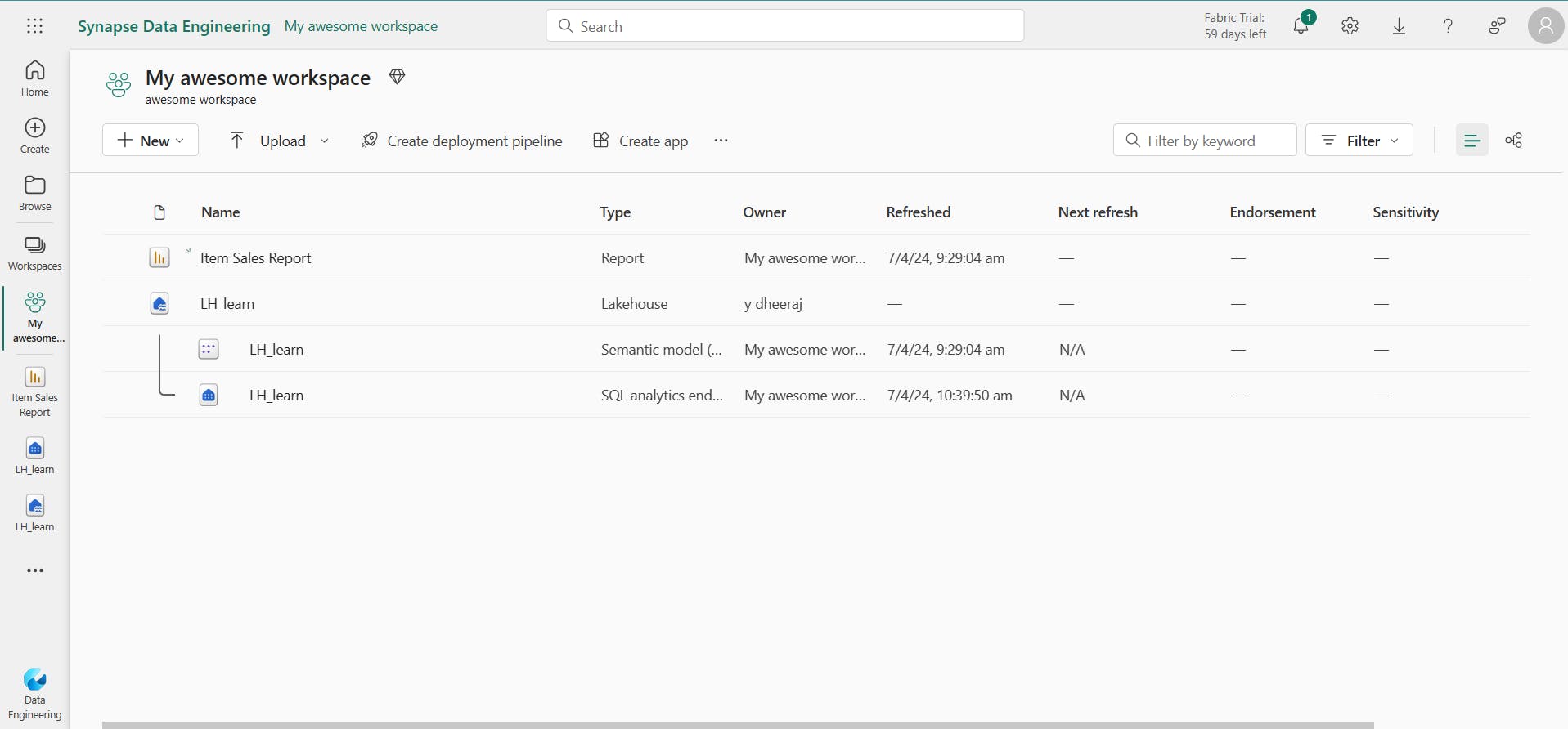
You create and configure a new lakehouse in the Data Engineering workload. Each L produces three named items in the Fabric-enabled workspace:
Lakehouse is the lakehouse storage and metadata, where you interact with files, folders, and table data.
Semantic model (default) is an automatically created data model based on the tables in the lakehouse. Power BI reports can be built from the semantic model.
SQL Endpoint is a read-only SQL endpoint through which you can connect and query data with Transact-SQL.
Shortcuts enable you to integrate data into your lakehouse while keeping it stored in external storage.
4. Ingest data into a lakehouse
There are many ways to load data into a Fabric lakehouse, including:
Upload: Upload local files or folders to the lakehouse. You can then explore and process the file data, and load the results into tables.
Dataflows (Gen2): Import and transform data from a range of sources using Power Query Online, and load it directly into a table in the lakehouse.
Notebooks: Use notebooks in Fabric to ingest and transform data, and load it into tables or files in the lakehouse.
Data Factory pipelines: Copy data and orchestrate data processing activities, loading the results into tables or files in the lakehouse.
5. Grant access to a lakehouse
Fabric lakehouse permissions are granted either at the workspace or item level.
You can also grant object-level security by using the SQL analytics endpoint to further control what users can access.
6. Explore and transform data in a lakehouse
After loading data into the lakehouse, you can use various tools and techniques to explore and transform it, including:
Apache Spark: Each Fabric lakehouse can use Spark pools through Notebooks or Spark Job Definitions to process data in files and tables in the lakehouse using Scala, PySpark, or Spark SQL.
Notebooks: Interactive coding interfaces in which you can use code to read, transform, and write data directly to the lakehouse as tables and/or files.
Spark job definitions: On-demand or scheduled scripts that use the Spark engine to process data in the lakehouse.
SQL analytic endpoint: Each lakehouse includes a SQL analytic endpoint through which you can run Transact-SQL statements to query, filter, aggregate, and otherwise explore data in lakehouse tables.
Dataflows (Gen2): In addition to using a dataflow to ingest data into the lakehouse, you can create a dataflow to perform subsequent transformations through Power Query, and optionally land transformed data back to the lakehouse.
Data pipelines: Orchestrate complex data transformation logic that operates on data in the lakehouse through a sequence of activities (such as dataflows, Spark jobs, and other control flow logic).
i. Analyze and visualize data in a lakehouse
The data in your lakehouse tables is included in a semantic model that defines a relational model for your data.
By combining the data visualization capabilities of Power BI with the centralized storage and tabular schema of a data lakehouse, you can implement an end-to-end analytics solution on a single platform.
7. Exercise - Create and ingest data with a Microsoft Fabric lakehouse
Create a Lakehouse
In this exercise, explore Microsoft Fabric lakehouse tasks like creating a lakehouse, importing data, querying tables with SQL, and generating reports. The exercise emphasizes the importance of the lakehouse as a central component in data engineering, warehousing, and analytics, enabling users to effectively manage and analyze their data within the lakehouse environment.
Large-scale data analytics solutions have traditionally been built around a data warehouse, in which data is stored in relational tables and queried using SQL. The growth in “big data” (characterized by high volumes, variety, and velocity of new data assets) together with the availability of low-cost storage and cloud-scale distributed compute technologies has led to an alternative approach to analytical data storage; the data lake.
In a data lake, data is stored as files without imposing a fixed schema for storage. Increasingly, data engineers and analysts seek to benefit from the best features of both of these approaches by combining them in a data lakehouse; in which data is stored in files in a data lake and a relational schema is applied to them as a metadata layer so that they can be queried using traditional SQL semantics.
In Microsoft Fabric, a lakehouse provides highly scalable file storage in a OneLake store (built on Azure Data Lake Store Gen2) with a metastore for relational objects such as tables and views based on the open source Delta Lake table format. Delta Lake enables you to define a schema of tables in your lakehouse that you can query using SQL.
i. Create a workspace
ii Create a lakehouse
iii. Upload a file
iv. Explore shortcuts
v. Load file data into a table
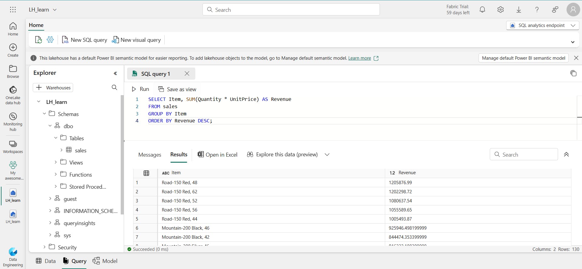
vi. Use SQL to query tables
SELECT Item, SUM(Quantity * UnitPrice) AS Revenue
FROM sales
GROUP BY Item
ORDER BY Revenue DESC;
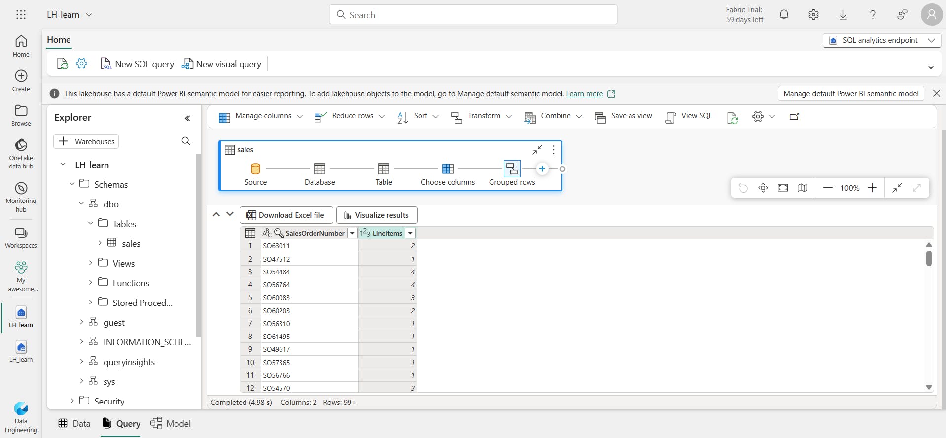
vii. Create a visual query
viii. Create a report
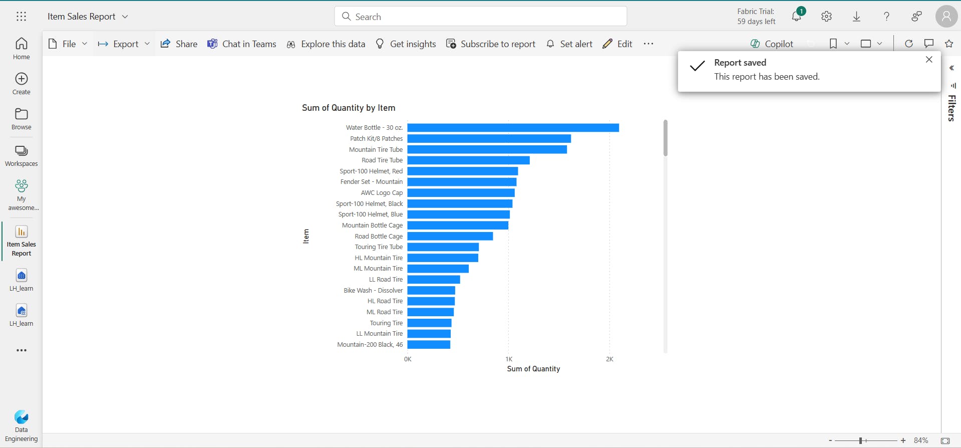
ix. Clean up resources
In this exercise, I have created a lakehouse and imported data into it.
I’ve seen how a lakehouse consists of files and tables stored in a OneLake data store.
The managed tables can be queried using SQL, and are included in a default semantic model to support data visualizations.
8. Knowledge check
What is a Microsoft Fabric lakehouse?
Lakehouses combine data lake and data warehouse features.
You want to include data in an external Azure Data Lake Store Gen2 location in your lakehouse, without the requirement to copy the data. What should you do?
A shortcut enables you to include external data in the lakehouse.
You want to use Apache Spark to interactively explore data in a file in the lakehouse. What should you do?
A notebook enables interactive Spark coding.
9. Summary
Microsoft Fabric lakehouses provide data engineers and analysts with the combined benefits of data lake storage and a relational data warehouse.
You can use a lakehouse as the basis of an end-to-end data analytics solution that includes data ingestion, transformation, modeling, and visualization.
Learning objectives
In this module, you'll learn how to:
Describe core features and capabilities of lakehouses in Microsoft Fabric
Create a lakehouse
Ingest data into files and tables in a lakehouse
Query lakehouse tables with SQL
build report
III. Use Apache Spark in Microsoft Fabric
Apache Spark is a core technology for large-scale data analytics.
Microsoft Fabric provides support for Spark clusters, enabling you to analyze and process data in a Lakehouse at scale.
1. Introduction
Apache Spark is an open-source parallel processing framework for large-scale data processing and analytics.
This module explores how you can use Spark in Microsoft Fabric to ingest, process, and analyze data in a lakehouse.
While the core techniques and code described in this module are common to all Spark implementations, the integrated tools and ability to work with Spark in the same environment as other data services in Microsoft Fabric makes it easier to incorporate Spark-based data processing into your overall data analytics solution.
2. Prepare to use Apache Spark
Apache Spark is a distributed data processing framework that enables large-scale data analytics by coordinating work across multiple processing nodes in a cluster.
Put more simply, Spark uses a "divide and conquer" approach to processing large volumes of data quickly by distributing the work across multiple computers.
The process of distributing tasks and collating results is handled for you by Spark.
i. Spark settings
In Microsoft Fabric, each workspace is assigned a Spark cluster.
ii. Libraries
3. Run Spark code
To edit and run Spark code in Microsoft Fabric, you can use notebooks, or you can define a Spark job.
i. Notebooks
When you want to use Spark to explore and analyze data interactively, use a notebook.
Notebooks enable you to combine text, images, and code written in multiple languages to create an interactive item that you can share with others and collaborate.
ii. Spark job definition
If you want to use Spark to ingest and transform data as part of an automated process, you can define a Spark job to run a script on-demand or based on a schedule.
4. Work with data in a Spark dataframe
Natively, Spark uses a data structure called a resilient distributed dataset (RDD); but while you can write code that works directly with RDDs, the most commonly used data structure for working with structured data in Spark is the dataframe, which is provided as part of the Spark SQL library.
i. Inferring a schema
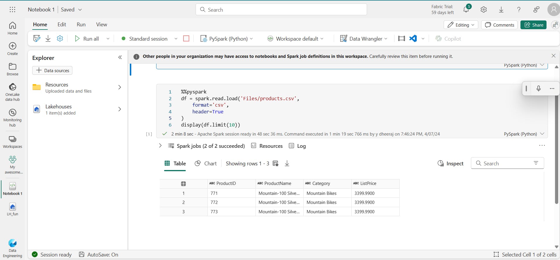
products.csv [Link]
%%pyspark
df = spark.read.load('Files/data/products.csv',
    format='csv',
    header=True
)
display(df.limit(10))
The %%pyspark line at the beginning is called a magic, and tells Spark that the language used in this cell is PySpark.
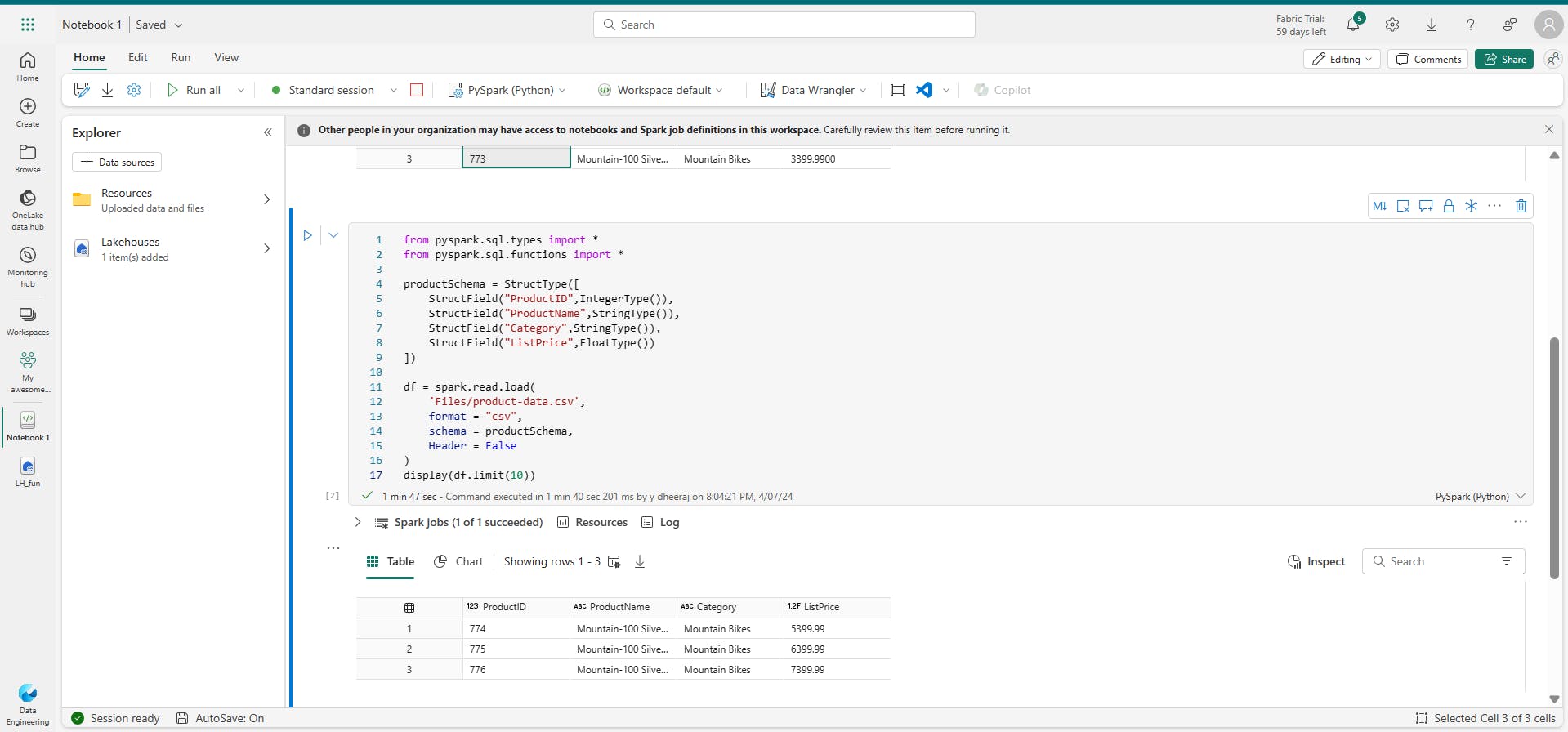
ii. Specifying an explicit schema
Specifying an explicit schema also improves performance!
from pyspark.sql.types import *
from pyspark.sql.functions import *

productSchema = StructType([
    StructField("ProductID",IntegerType()),
    StructField("ProductName",StringType()),
    StructField("Category",StringType()),
    StructField("ListPrice",FloatType())
])

df = spark.read.load(
    'Files/product-data.csv',
    format = "csv",
    schema = productSchema,
    Header = False
)
display(df.limit(10))
iii. Filtering and grouping dataframes
pricelist_df = df.select("ProductID", "ListPrice")
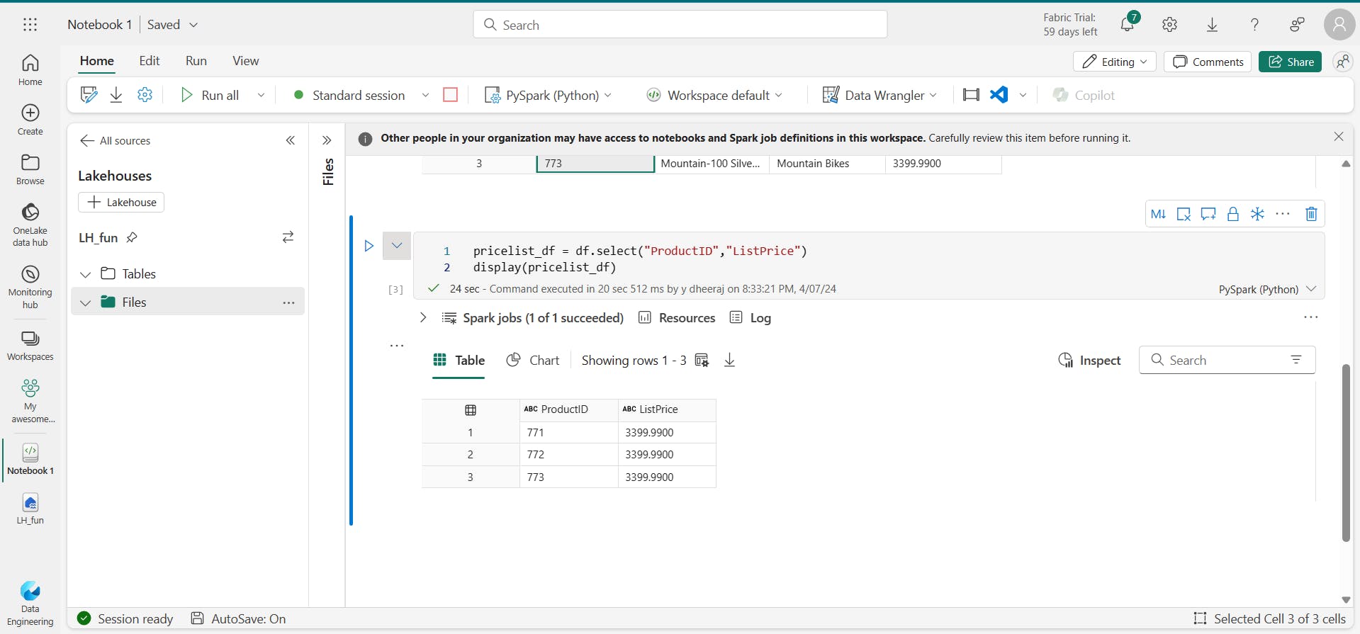
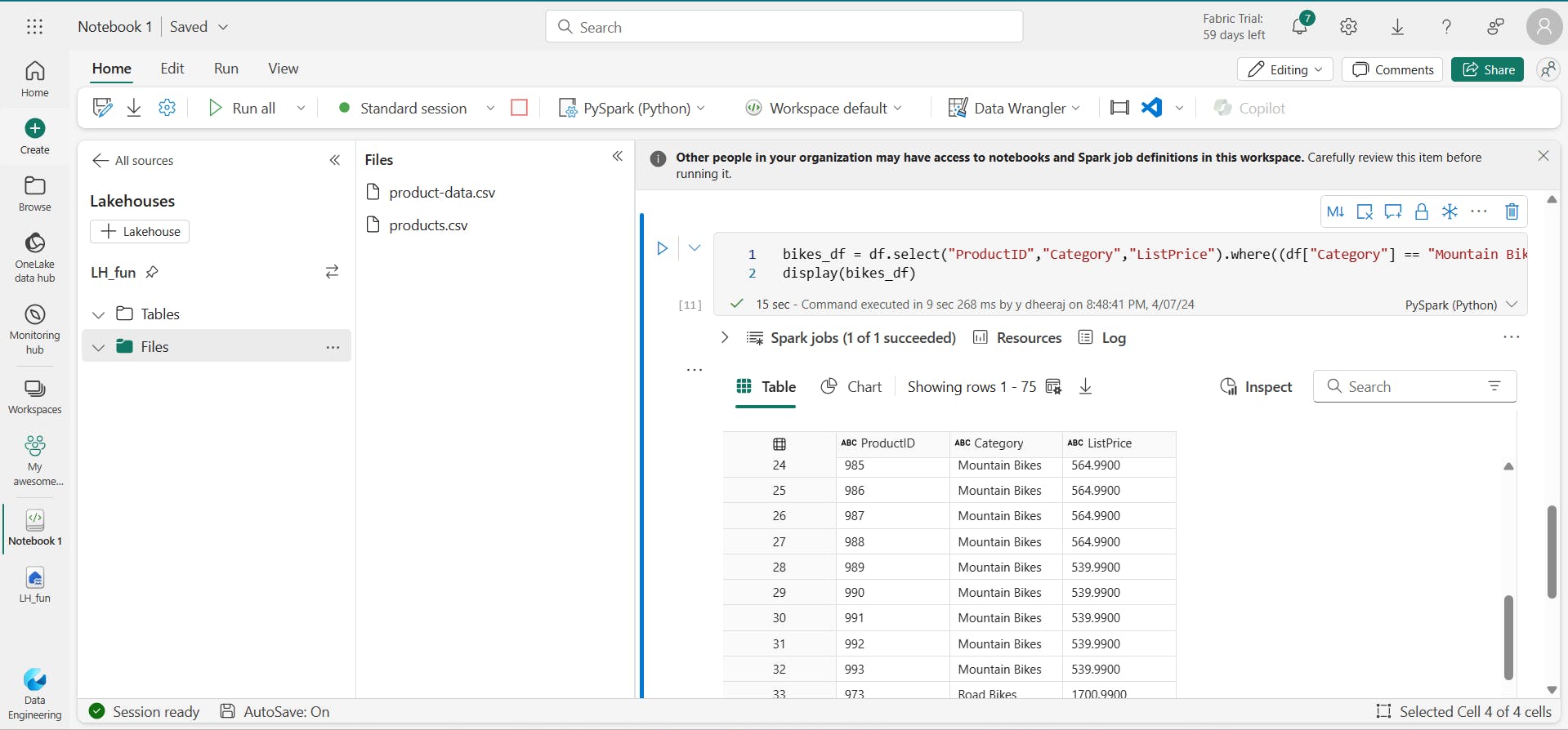
this example code chains the select and where methods to create a new dataframe containing the ProductName and ListPrice columns for products with a category of Mountain Bikes or Road Bikes:
bikes_df = df.select("ProductName", "Category", "ListPrice").where((df["Category"]=="Mountain Bikes") | (df["Category"]=="Road Bikes"))
display(bikes_df)
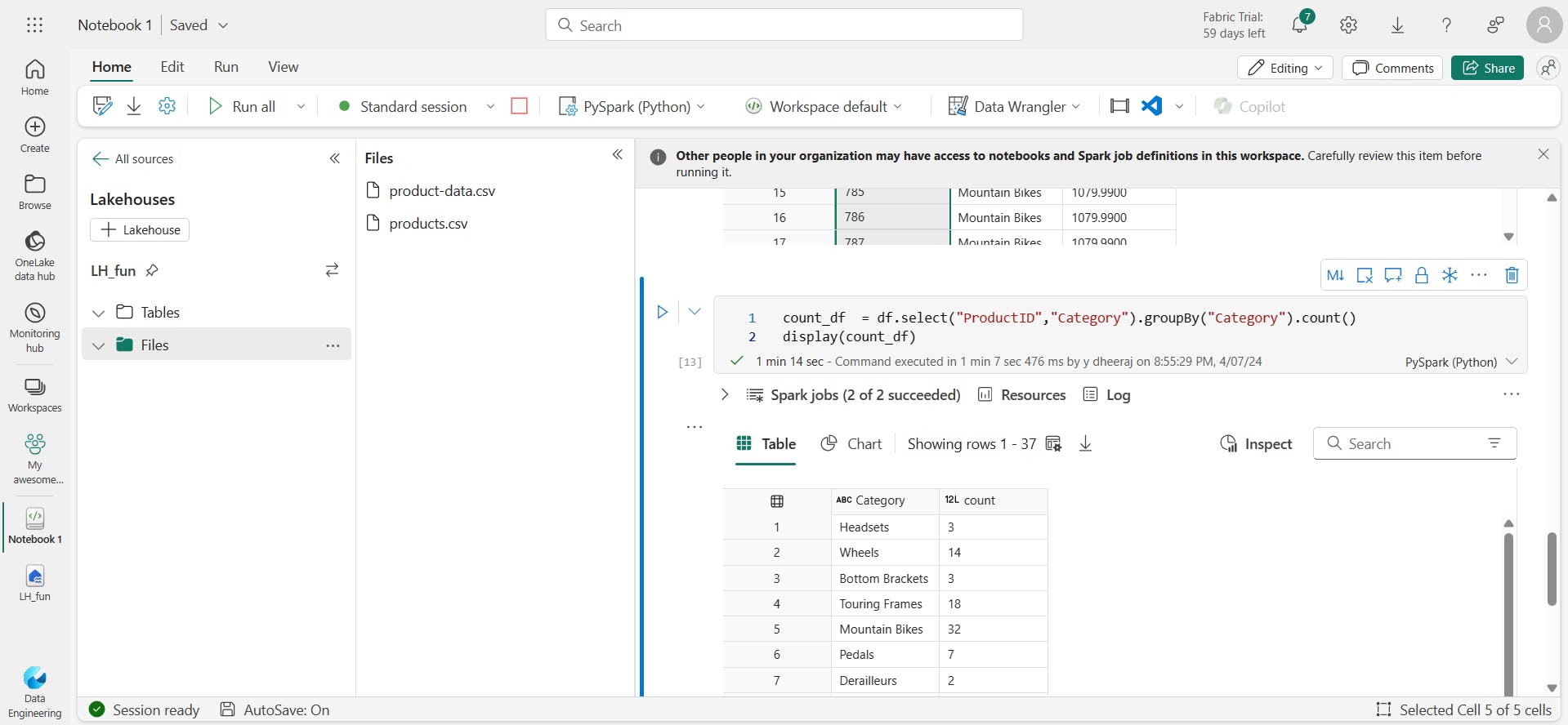
PySpark code counts the number of products for each category:
count_df  = df.select("ProductID","Category").groupBy("Category").count()
display(count_df)
iv. Saving a dataframe
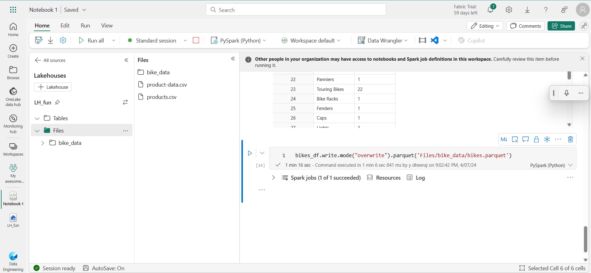
You'll often want to use Spark to transform raw data and save the results for further analysis or downstream processing. The following code example saves the dataFrame into a parquet file in the data lake, replacing any existing file of the same name.
bikes_df.write.mode("overwrite").parquet('Files/bike_data/bikes.parquet')
v. Partitioning the output file
Partitioning is an optimization technique that enables Spark to maximize performance across the worker nodes. More performance gains can be achieved when filtering data in queries by eliminating unnecessary disk IO.
bikes_df.write.partitionBy("Category").mode("overwrite").parquet("Files/bike_data")
vi. Load partitioned data
road_bikes_df = spark.read.parquet('Files/bike_data/Category=Road Bikes')
display(road_bikes_df.limit(5))
5. Work with data using Spark SQL
The Dataframe API is part of a Spark library named Spark SQL, which enables data analysts to use SQL expressions to query and manipulate data.
i. Creating database objects in the Spark catalog
df.createOrReplaceTempView("products_view")
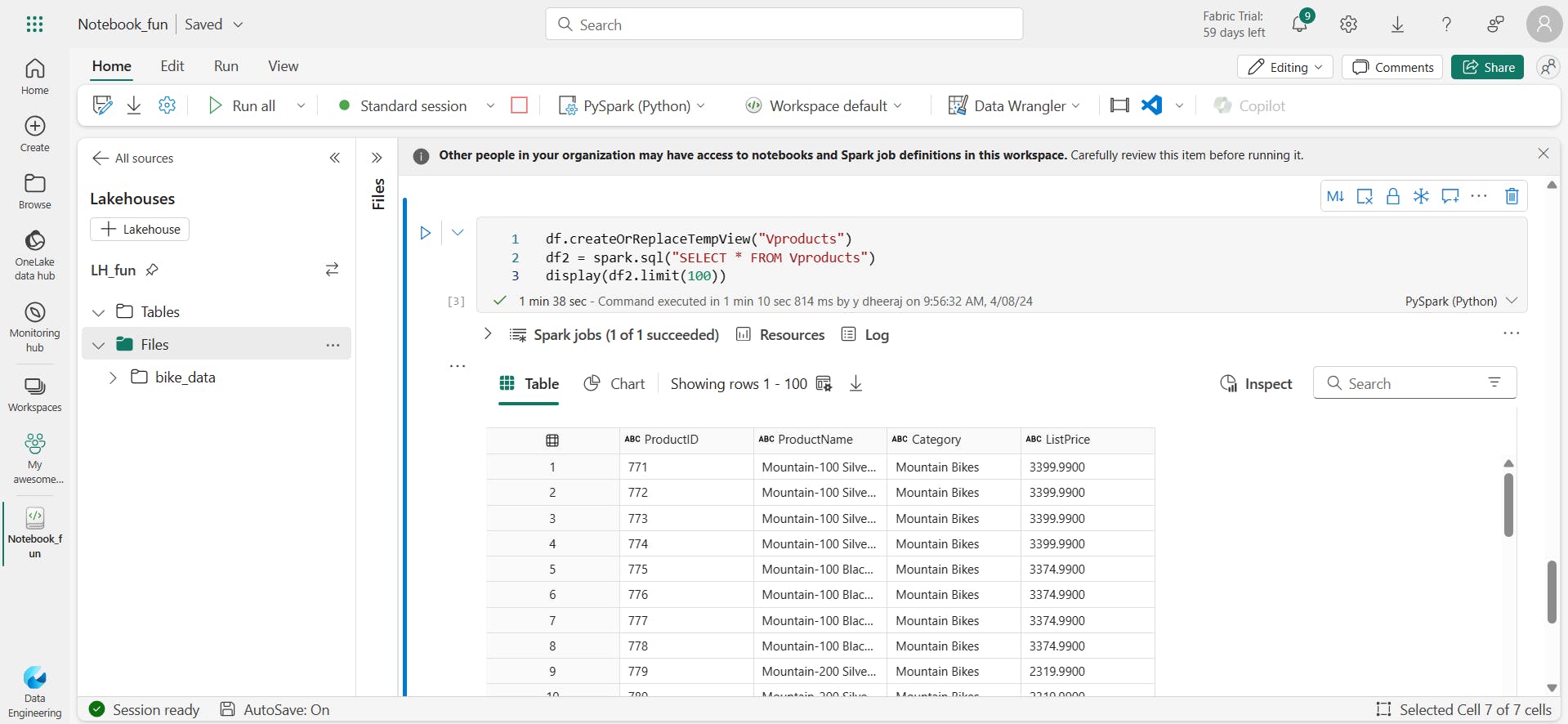
df.createOrReplaceTempView("Vproducts")
df2 = spark.sql("SELECT * FROM Vproducts")
display(df2)
You can create an empty table by using the spark.catalog.createTable method, or you can save a dataframe as a table by using its saveAsTable method. Deleting a managed table also deletes its underlying data.
spark.catalog.createTable("tEmpty",schema = spark.range(1).schema, source = 'parquet')
spark.catalog.listTables()

spark.sql("DROP TABLE tEmpty")
above code skipped taking >50 min time.
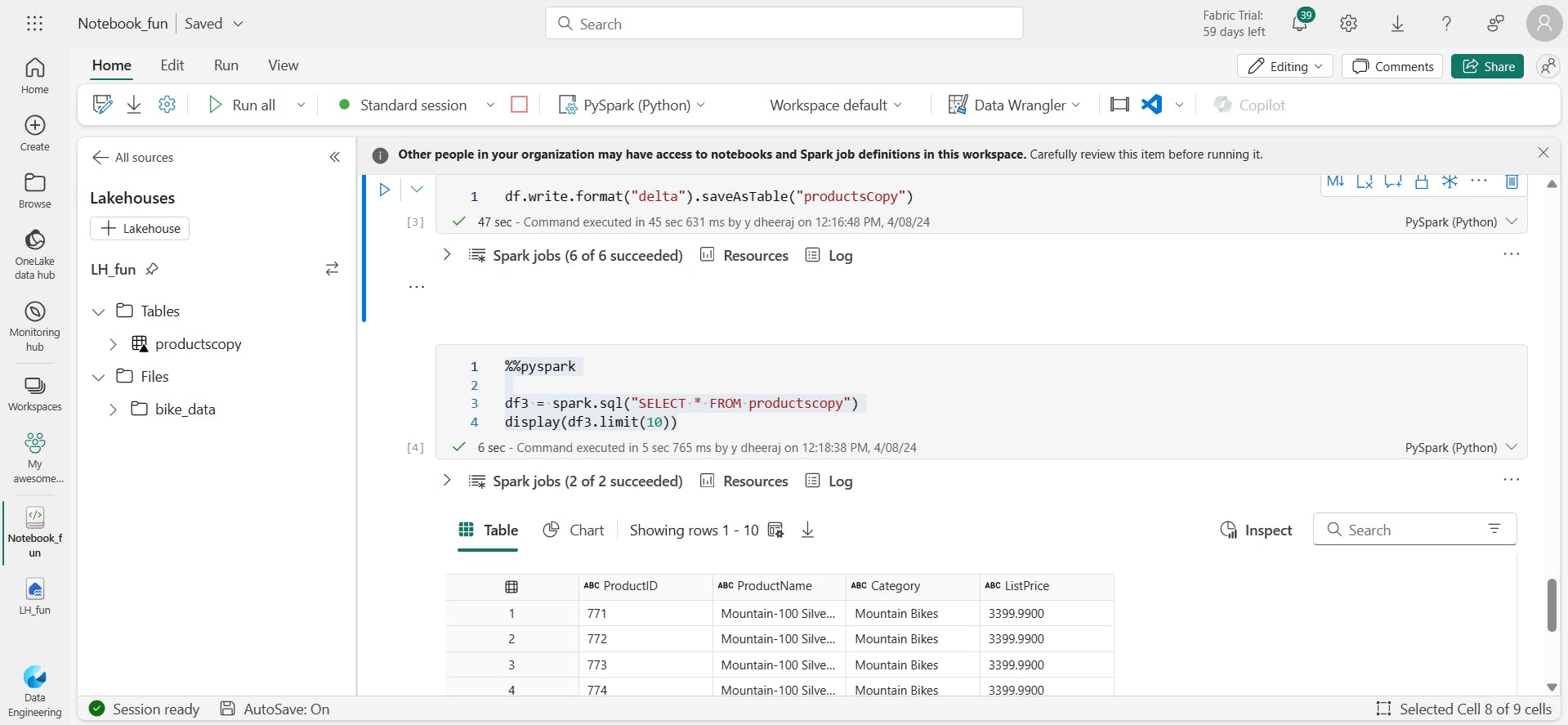
For example, the following code saves a dataframe as a new table named products:
df.write.format("delta").saveAsTable("products")
%%pyspark

df3 = spark.sql("SELECT * FROM productscopy")
display(df3.limit(10))
Delta tables support features commonly found in relational database systems, including transactions, versioning, and support for streaming data.
Additionally, you can create external tables by using the spark.catalog.createExternalTable method. External tables define metadata in the catalog but get their underlying data from an external storage location; typically a folder in the Files storage area of a lakehouse. Deleting an external table doesn't delete the underlying data.
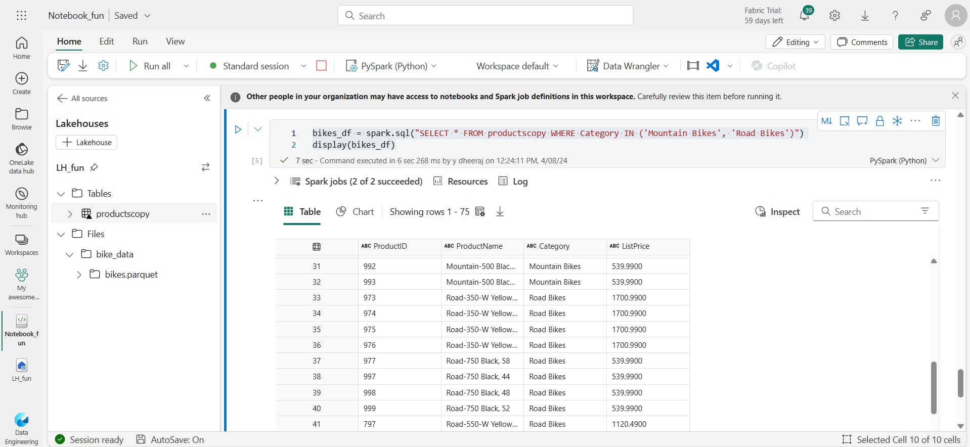
ii. Using the Spark SQL API to query data
bikes_df = spark.sql("SELECT * FROM productscopy WHERE Category IN ('Mountain Bikes', 'Road Bikes')")
display(bikes_df)
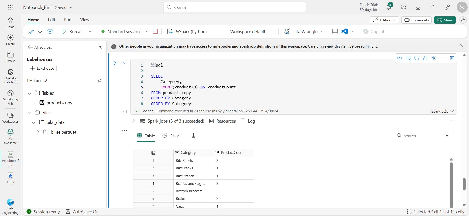
iii. Using SQL code
%%sql

SELECT
    Category,
    COUNT(ProductID) AS ProductCount
FROM productscopy
GROUP BY Category
ORDER BY Category
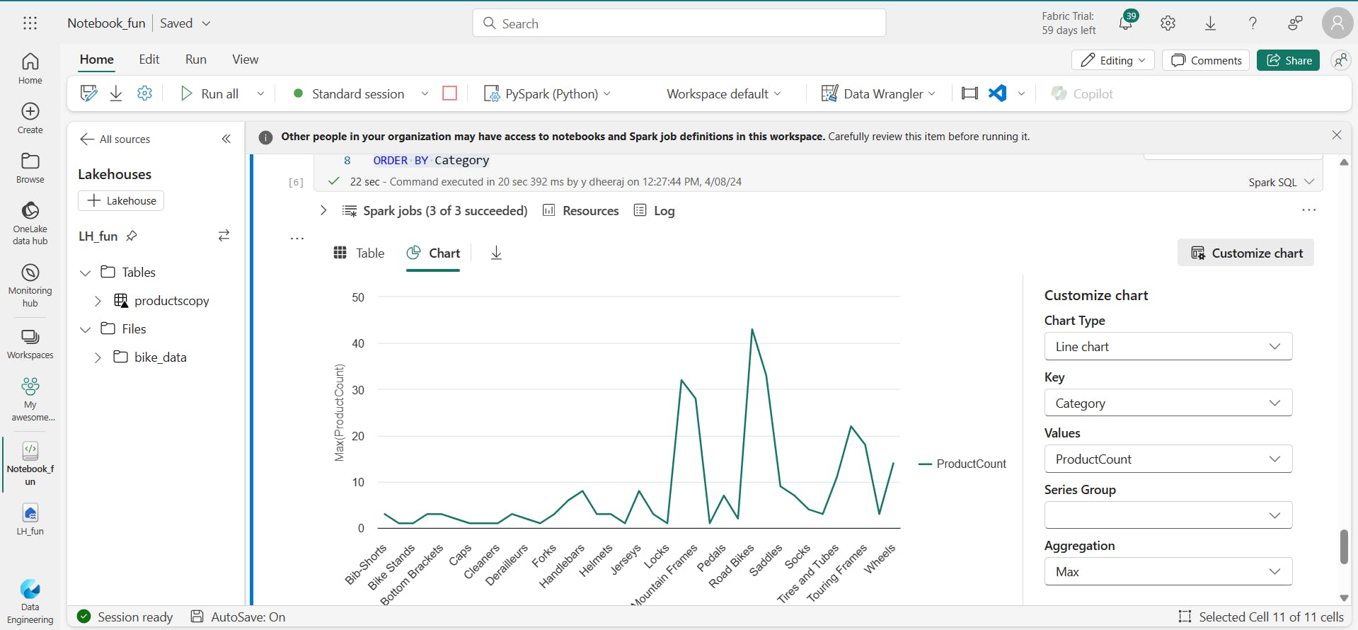
6. Visualize data in a Spark notebook
i. Using built-in notebook charts
ii. Using graphics packages in code
from matplotlib import pyplot as plt

# Get the data as a Pandas dataframe
data = spark.sql("SELECT Category, COUNT(ProductID) AS ProductCount \
                  FROM products \
                  GROUP BY Category \
                  ORDER BY Category").toPandas()

# Clear the plot area
plt.clf()

# Create a Figure
fig = plt.figure(figsize=(12,8))

# Create a bar plot of product counts by category
plt.bar(x=data['Category'], height=data['ProductCount'], color='orange')

# Customize the chart
plt.title('Product Counts by Category')
plt.xlabel('Category')
plt.ylabel('Products')
plt.grid(color='#95a5a6', linestyle='--', linewidth=2, axis='y', alpha=0.7)
plt.xticks(rotation=70)

# Show the plot area
plt.show()
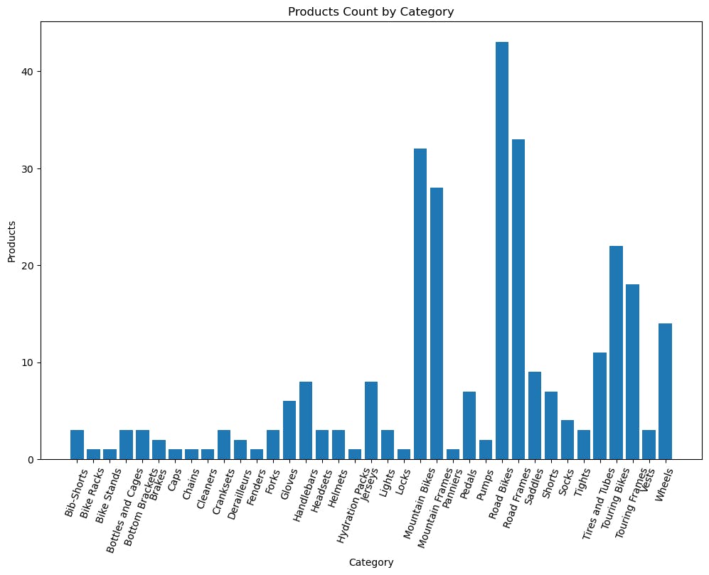
from matplotlib import pyplot as plt

# Get the data as a Pandas dataframe
data = spark.sql("SELECT Category, COUNT(ProductID) AS ProductCount FROM productscopy GROUP BY Category ORDER BY Category").toPandas()

# Clear the plot area
plt.clf()

# Create a Figure
fig = plt.figure(figsize=(12,8))

# Create a bar plot of product counts by category
plt.bar(x = data["Category"], height = data["ProductCount"])

# Customize the chart
plt.title("Products Count by Category")
plt.xlabel("Category")
plt.ylabel("Products")
plt.xticks(rotation=70)

# Show the plot area
plt.show()
7. Exercise - Analyze data with Apache Spark
i. Create a lakehouse and upload files

ii. Create a notebook
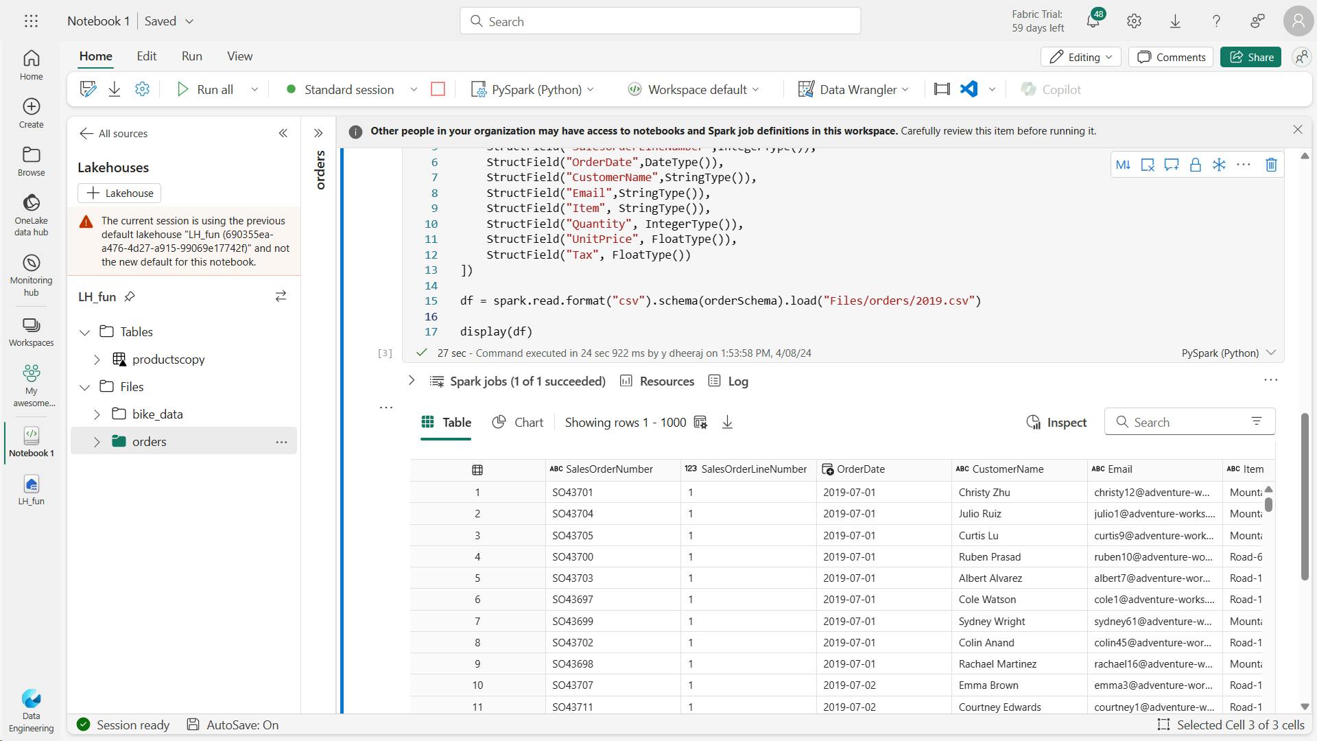
iii. Load data into a dataframe
from pyspark.sql.types import *

orderSchema = StructType([
    StructField("SalesOrderNumber", StringType()),
    StructField("SalesOrderLineNumber",IntegerType()),
    StructField("OrderDate",DateType()),
    StructField("CustomerName",StringType()),
    StructField("Email",StringType()),
    StructField("Item", StringType()),
    StructField("Quantity", IntegerType()),
    StructField("UnitPrice", FloatType()),
    StructField("Tax", FloatType())
])

df = spark.read.format("csv").schema(orderSchema).load("Files/orders/2019.csv")

display(df)
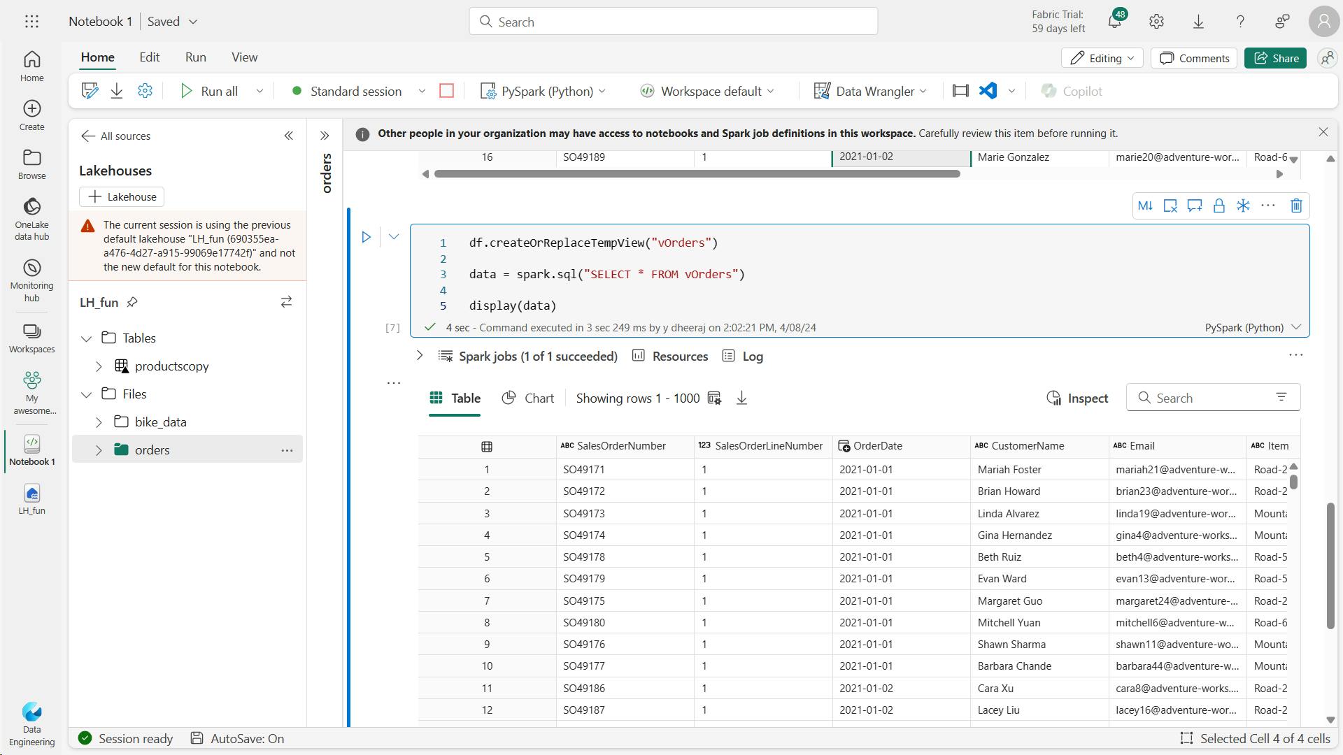
Create view:
df.createOrReplaceTempView("vOrders")

data = spark.sql("SELECT * FROM vOrders")

display(data)
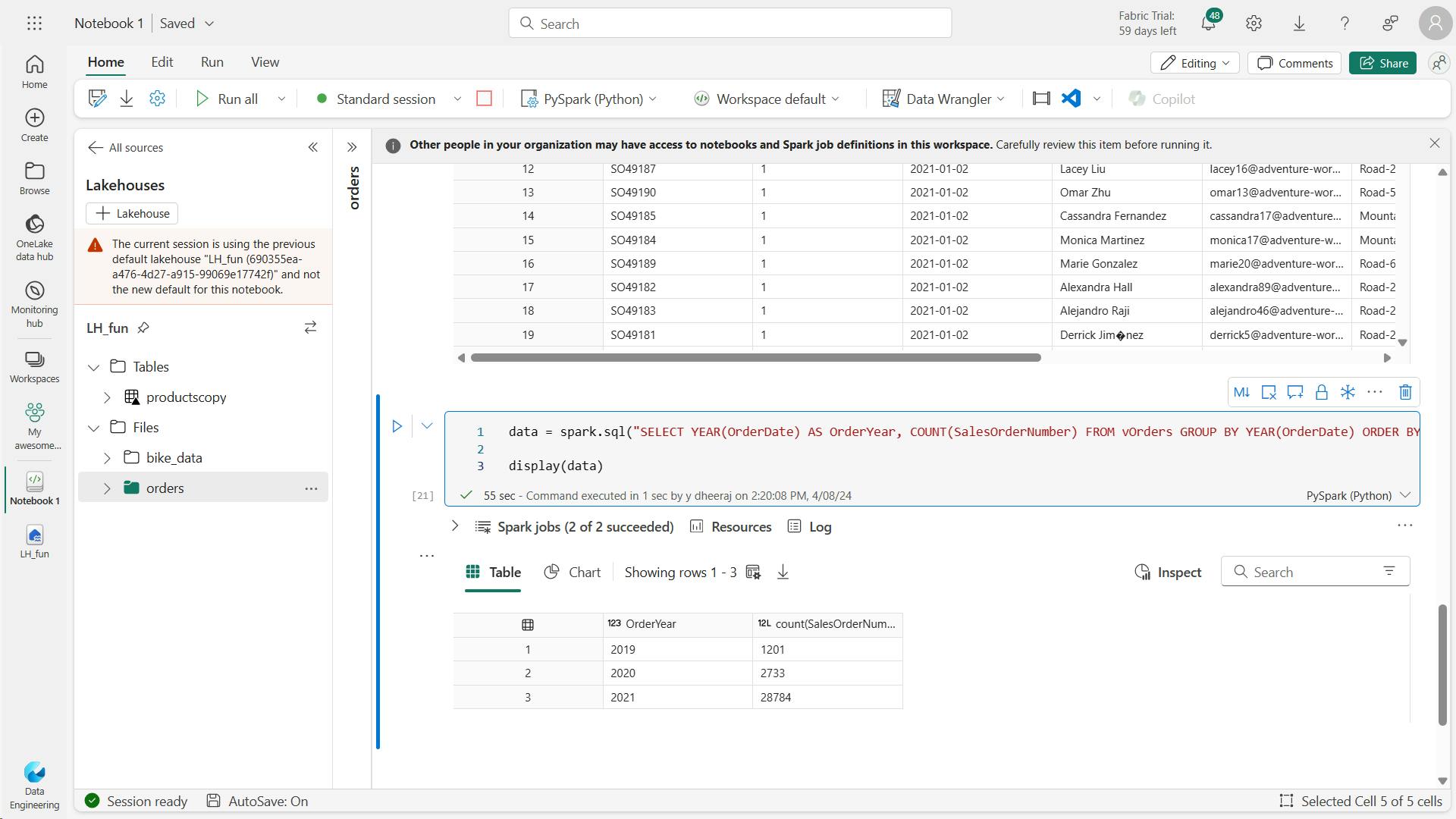
count:
data = spark.sql("SELECT YEAR(OrderDate) AS OrderYear, COUNT(SalesOrderNumber) FROM vOrders GROUP BY YEAR(OrderDate) ORDER BY YEAR(OrderDate)")

display(data)
iv. Explore data in a dataframe
a. Filter a dataframe
customers = df["CustomerName","Email"]

print(customers.count())
print(customers.distinct().count())
display(customers.distinct())

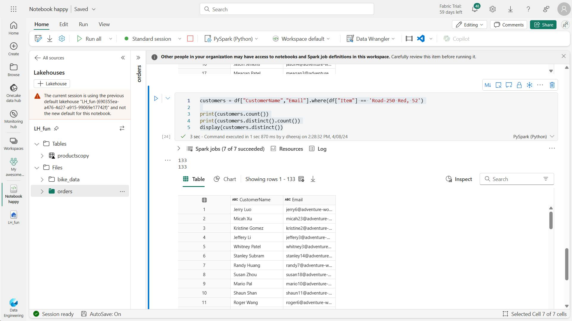
customers = df["CustomerName","Email"].where(df["Item"] == 'Road-250 Red, 52')

print(customers.count())
print(customers.distinct().count())
display(customers.distinct())
b. Aggregate and group data in a dataframe:
yearlySales = df.select(year(col("OrderDate")).alias("Year")).groupBy("Year").count().orderBy("Year")
display(yearlySales)

v. Use Spark to transform data files
a. Use dataframe methods and functions to transform data
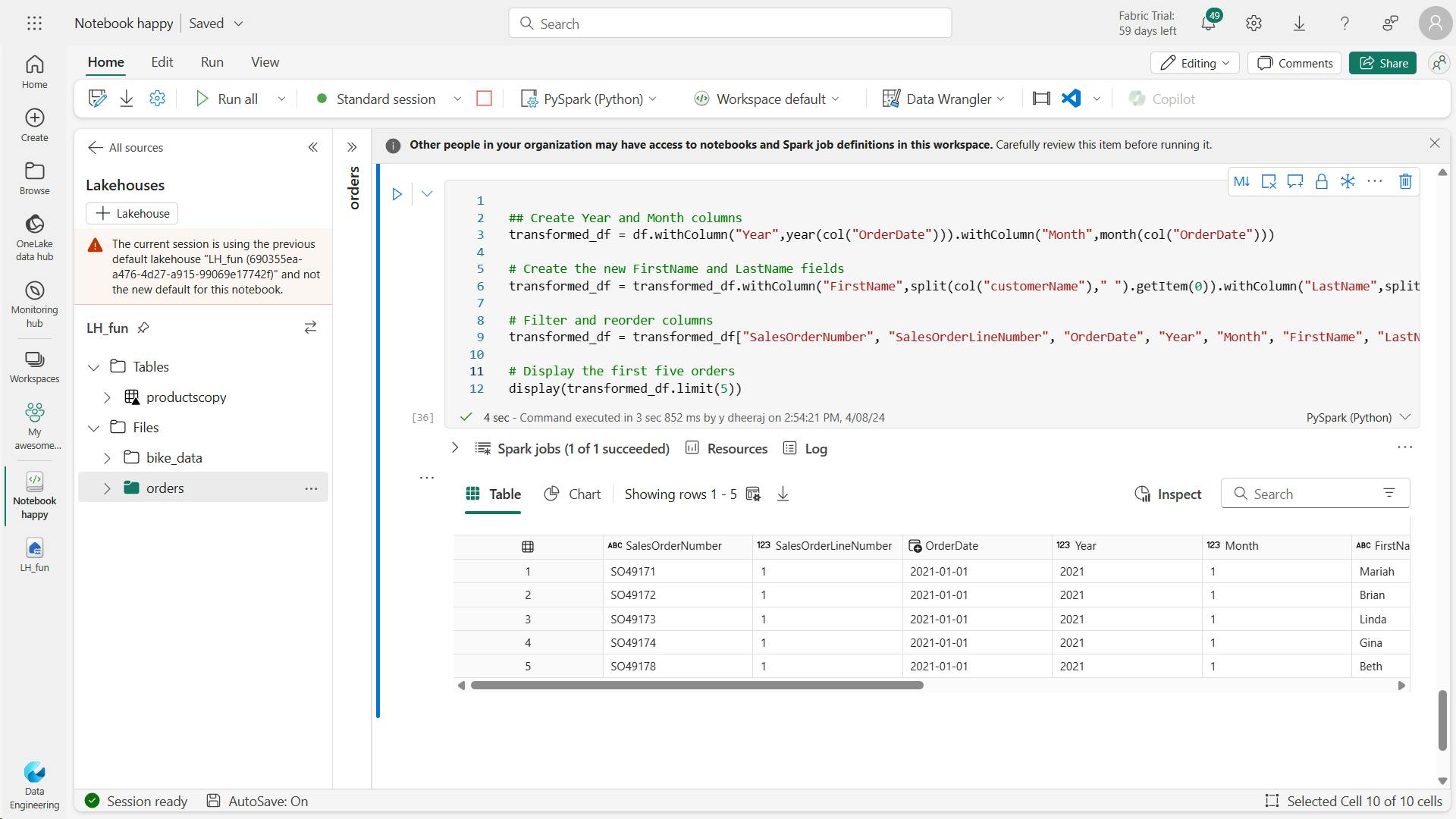
## Create Year and Month columns
transformed_df = df.withColumn("Year",year(col("OrderDate"))).withColumn("Month",month(col("OrderDate")))

# Create the new FirstName and LastName fields
transformed_df = transformed_df.withColumn("FirstName",split(col("customerName")," ").getItem(0)).withColumn("LastName",split(col("customerName")," ").getItem(1))

# Filter and reorder columns
transformed_df = transformed_df["SalesOrderNumber", "SalesOrderLineNumber", "OrderDate", "Year", "Month", "FirstName", "LastName", "Email", "Item", "Quantity", "UnitPrice", "Tax"]

# Display the first five orders
display(transformed_df.limit(5))
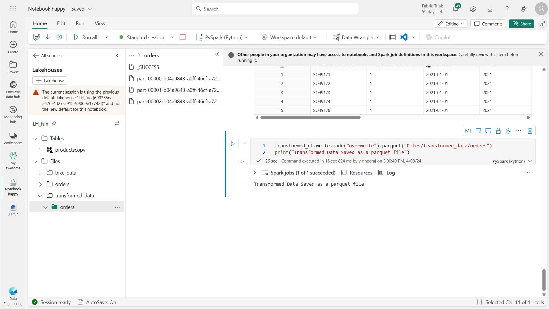
b. Save the transformed data
transformed_df.write.mode("overwrite").parquet("Files/transformed_data/orders")
print("Transformed Data Saved as a parquet file")
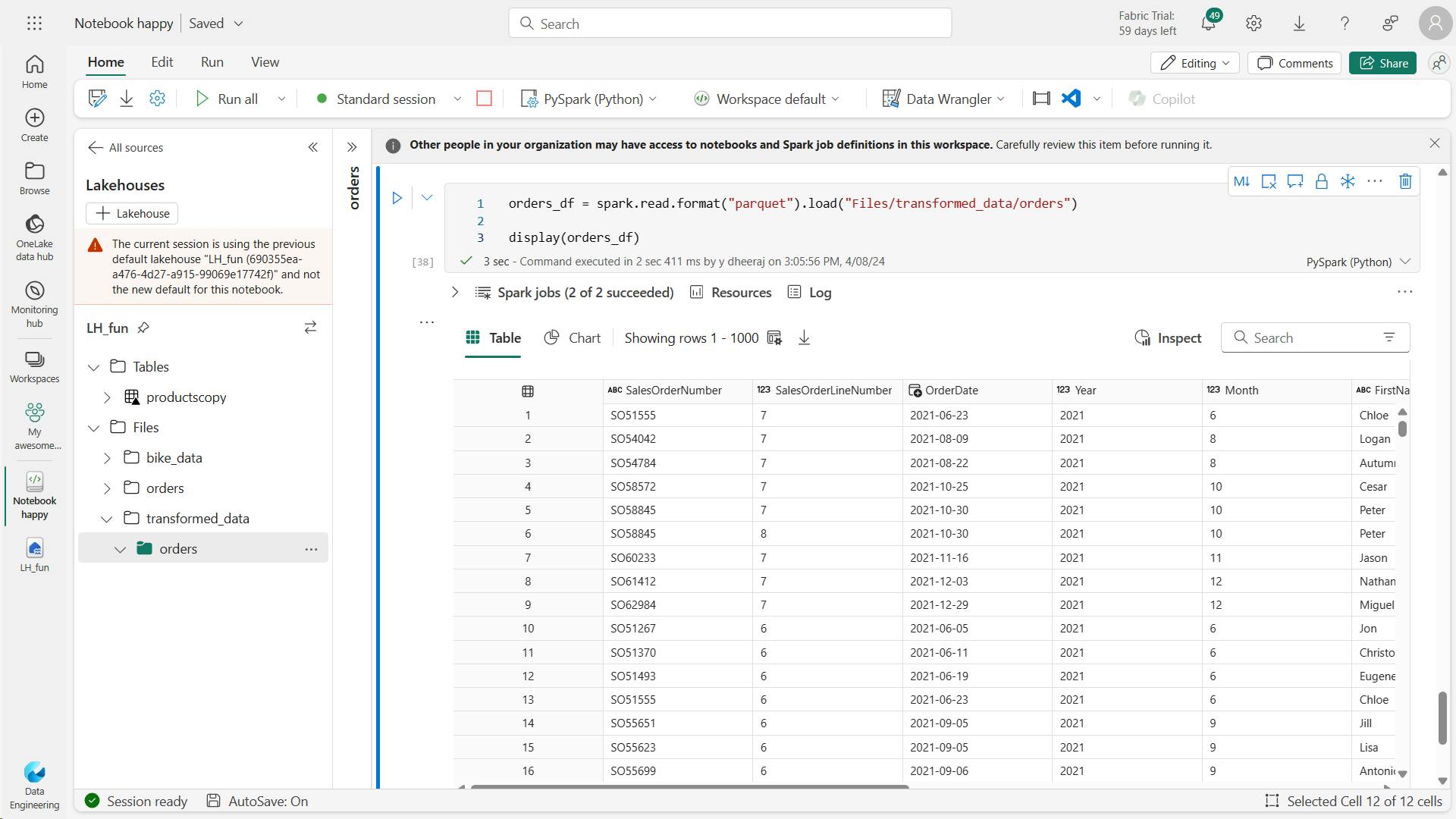
orders_df = spark.read.format("parquet").load("Files/transformed_data/orders")

display(orders_df)
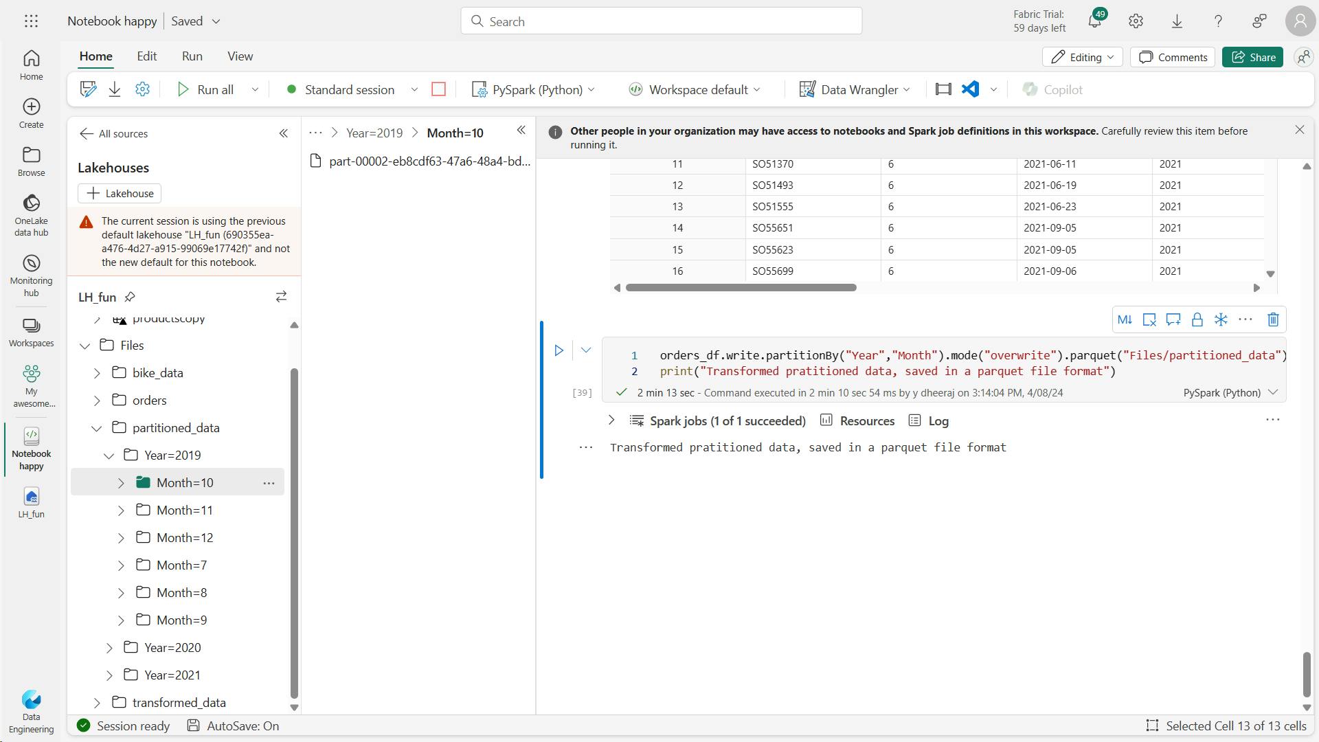
c. Save data in partitioned files
orders_df.write.partitionBy("Year","Month").mode("overwrite").parquet("Files/partitioned_data")
print("Transformed pratitioned data, saved in a parquet file format")
orders_2021_df = spark.read.format("parquet").load("Files/partitioned_data/Year=2021/Month=*")
display(orders_2021_df)
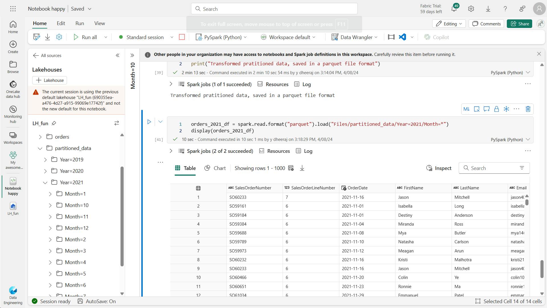
Note that the partitioning columns specified in the path (Year and Month) are not included in the dataframe.
vi. Work with tables and SQL
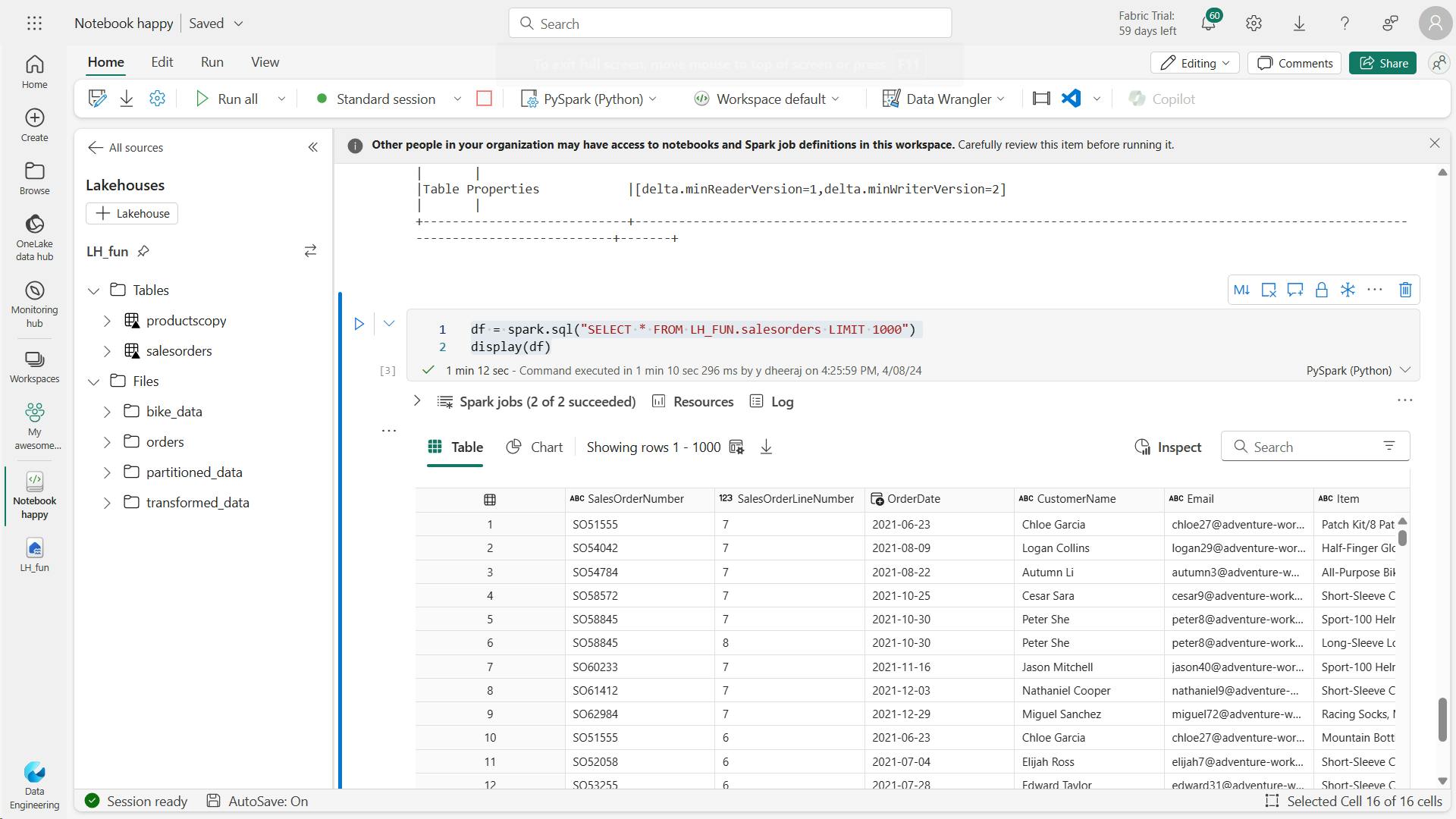
a. Create a table
spark.sql("DROP TABLE salesorders")

df.write.format("delta").saveAsTable("salesorders")

spark.sql("DESCRIBE EXTENDED salesorders").show(truncate=False)

df = spark.sql("SELECT * FROM [your_lakehouse].salesorders LIMIT 1000")
display(df)
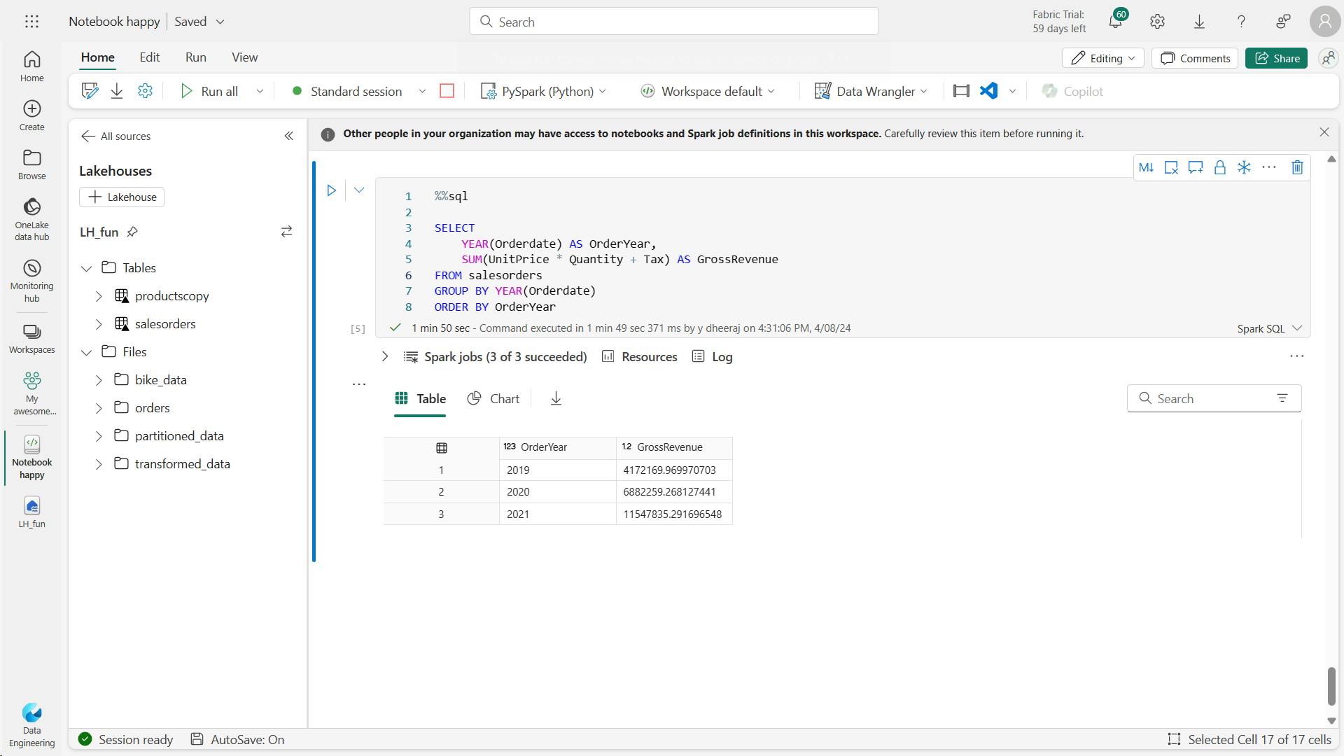
b. Run SQL code in a cell
%%sql
SELECT YEAR(OrderDate) AS OrderYear,
       SUM((UnitPrice * Quantity) + Tax) AS GrossRevenue
FROM salesorders
GROUP BY YEAR(OrderDate)
ORDER BY OrderYear;
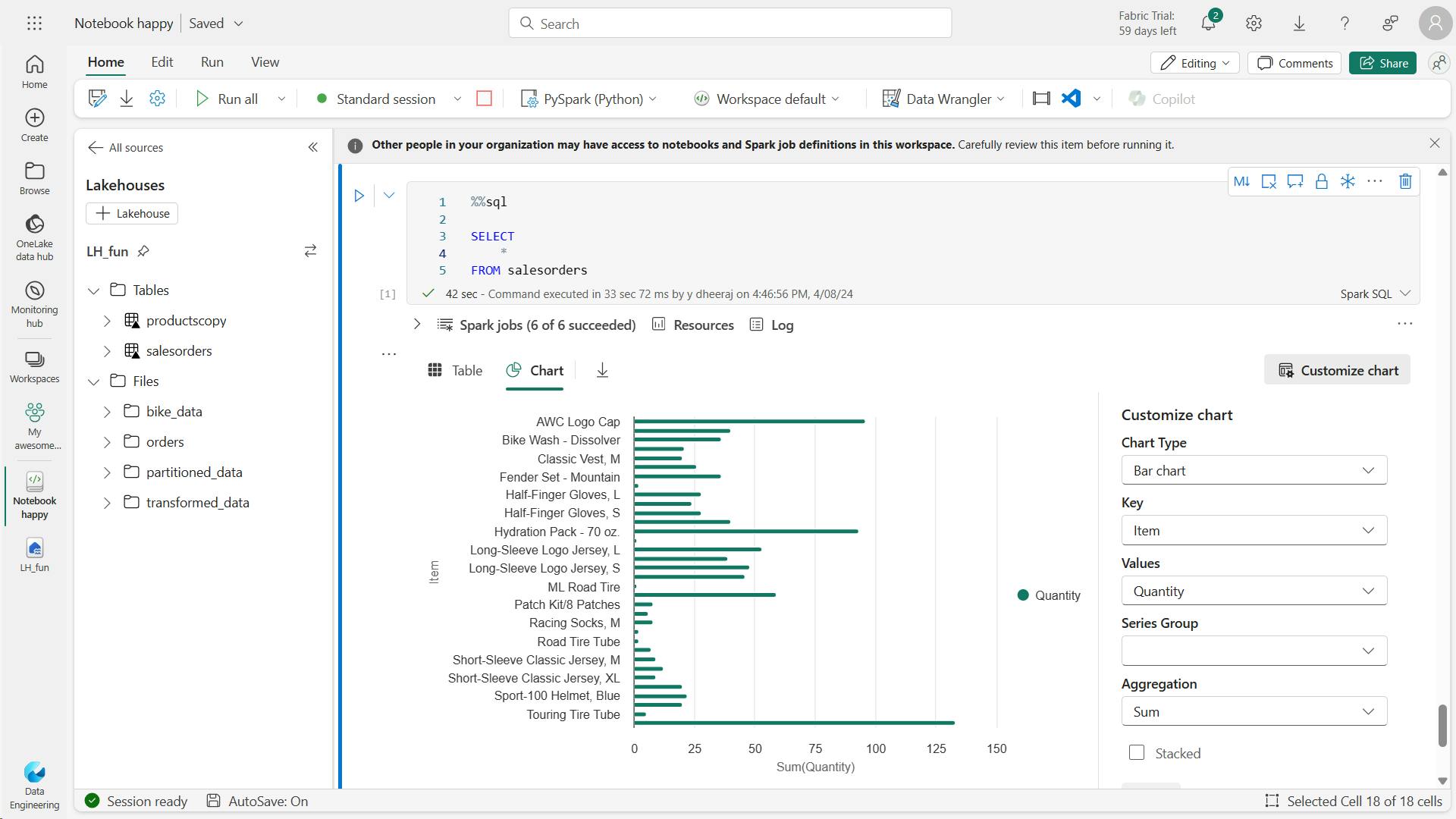
vii. Visualize data with Spark
%%sql

SELECT
    *
FROM salesorders
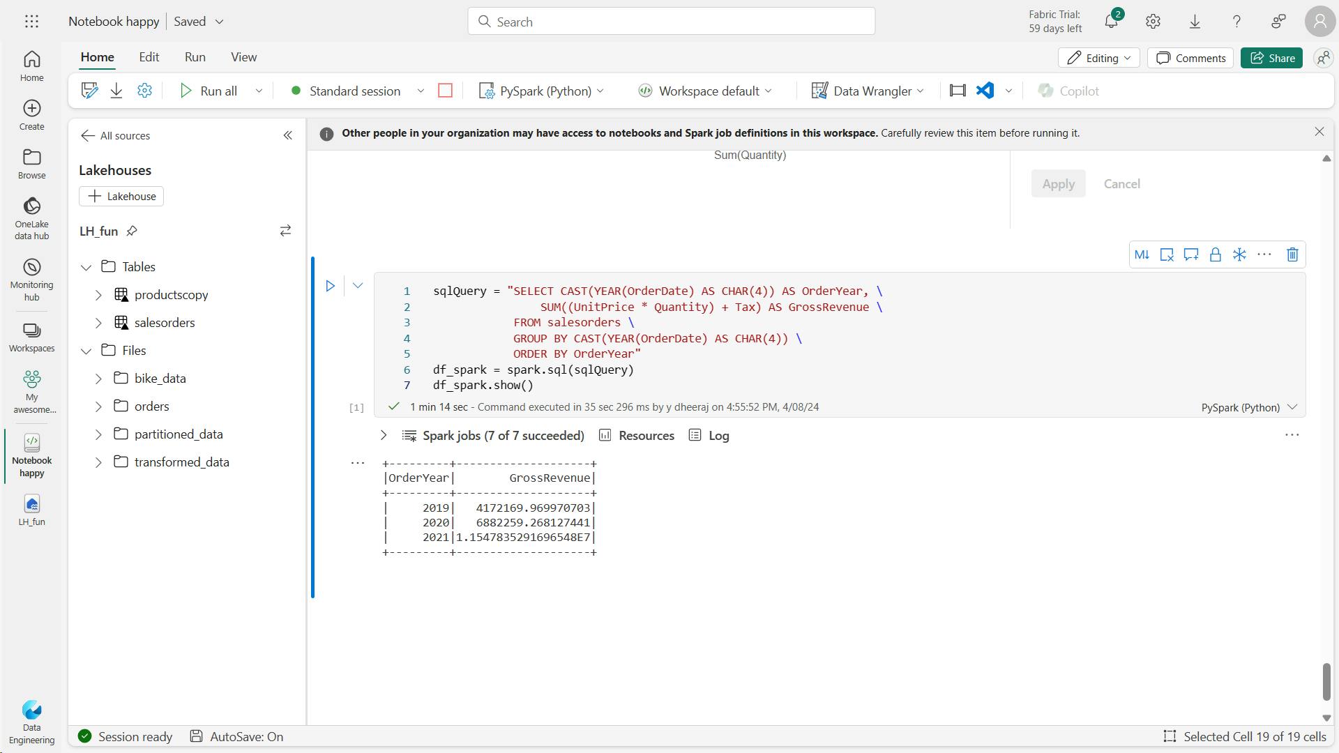
a. Get started with matplotlib
sqlQuery = "SELECT CAST(YEAR(OrderDate) AS CHAR(4)) AS OrderYear, \
                SUM((UnitPrice * Quantity) + Tax) AS GrossRevenue \
            FROM salesorders \
            GROUP BY CAST(YEAR(OrderDate) AS CHAR(4)) \
            ORDER BY OrderYear"
df_spark = spark.sql(sqlQuery)
df_spark.show()
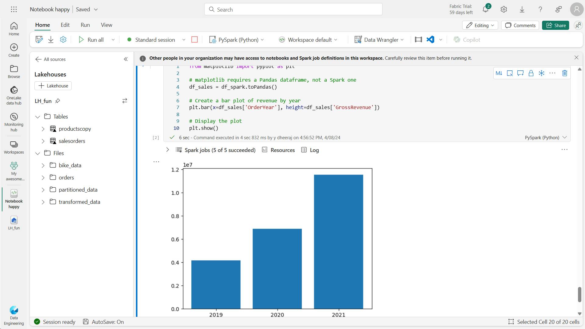
from matplotlib import pyplot as plt

# matplotlib requires a Pandas dataframe, not a Spark one
df_sales = df_spark.toPandas()

# Create a bar plot of revenue by year
plt.bar(x=df_sales['OrderYear'], height=df_sales['GrossRevenue'])

# Display the plot
plt.show()
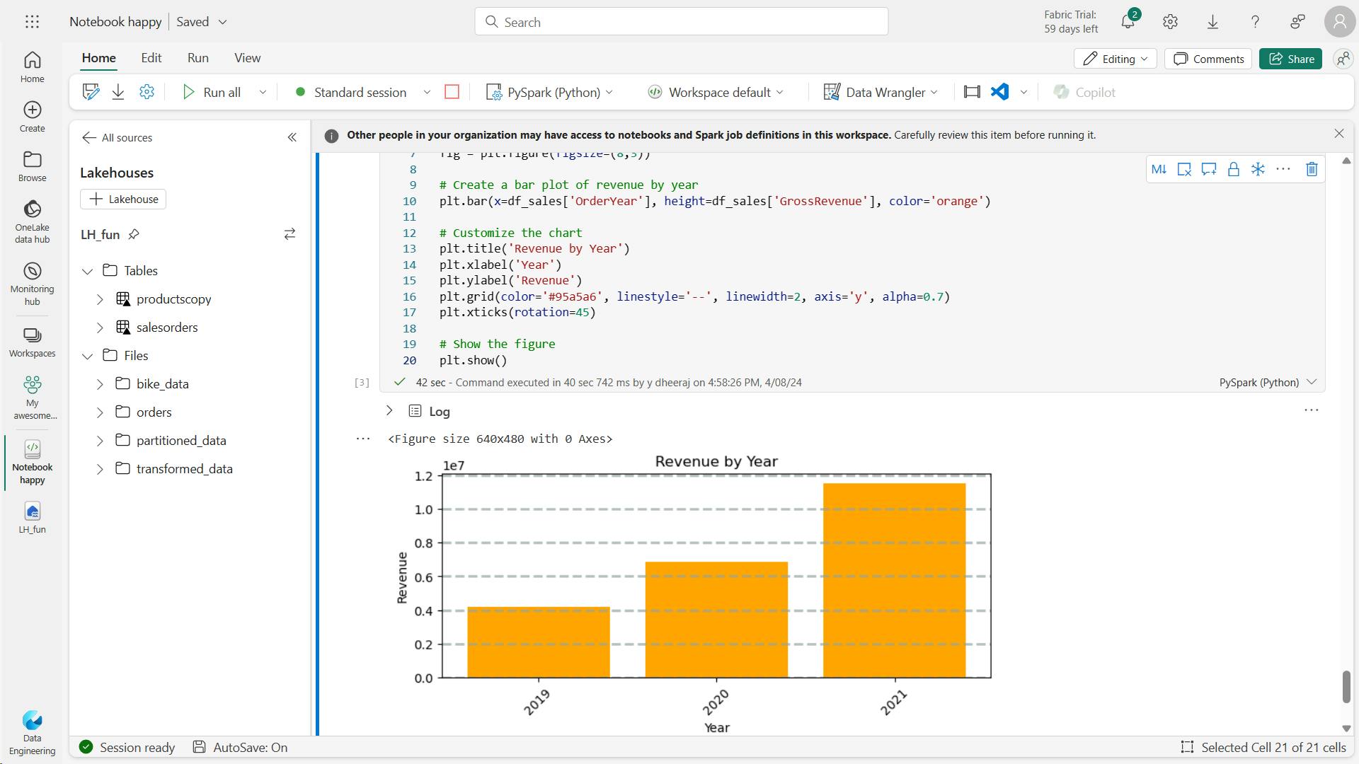
from matplotlib import pyplot as plt

# Clear the plot area
plt.clf()

# Create a Figure
fig = plt.figure(figsize=(8,3))

# Create a bar plot of revenue by year
plt.bar(x=df_sales['OrderYear'], height=df_sales['GrossRevenue'], color='orange')

# Customize the chart
plt.title('Revenue by Year')
plt.xlabel('Year')
plt.ylabel('Revenue')
plt.grid(color='#95a5a6', linestyle='--', linewidth=2, axis='y', alpha=0.7)
plt.xticks(rotation=45)

# Show the figure
plt.show()
from matplotlib import pyplot as plt
# Clear the plot area
plt.clf()
# Create a figure for 2 subplots (1 row, 2 columns)
fig, ax = plt.subplots(1, 2, figsize = (10,4))
# Create a bar plot of revenue by year on the first axis
ax[0].bar(x=df_sales['OrderYear'], height=df_sales['GrossRevenue'], color='orange')
ax[0].set_title('Revenue by Year')
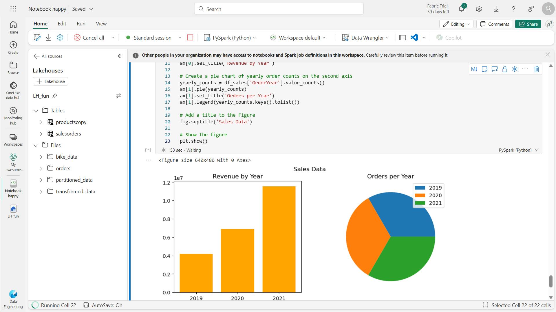
# Create a pie chart of yearly order counts on the second axis
yearly_counts = df_sales['OrderYear'].value_counts()
ax[1].pie(yearly_counts)
ax[1].set_title('Orders per Year')
ax[1].legend(yearly_counts.keys().tolist())
# Add a title to the Figure
fig.suptitle('Sales Data')
# Show the figure
plt.show()
b. Use the seaborn library
viii. Save the notebook and end the Spark session
ix. Clean up resources
8. Knowledge check
You want to use Apache Spark to explore data interactively in Microsoft Fabric. What should you create?
Notebooks enable you to run Spark code interactively.
You need to use Spark to analyze data in a CSV file. What's the simplest way to accomplish this goal?
You can load data from files in many formats, including CSV, into a Spark dataframe.
Which method is used to split the data across folders when saving a dataframe?
The partitionBy method partitions the dataframe based on specified columns.
9. Summary
Apache Spark is a key technology used in big data analytics.
Spark support in Microsoft Fabric enables you to integrate big data processing in Spark with the other data analytics and visualization capabilities of the platform.
Learning objectives
In this module, you'll learn how to:
Configure Spark in a Microsoft Fabric workspace
Identify suitable scenarios for Spark notebooks and Spark jobs
Use Spark dataframes to analyze and transform data
Use Spark SQL to query data in tables and views
Visualize data in a Spark notebook
IV. Work with Delta Lake tables in Microsoft Fabric
Tables in a Microsoft Fabric lakehouse are based on the Delta Lake storage format commonly used in Apache Spark. By using the enhanced capabilities of delta tables, you can create advanced analytics solutions.
1. Introduction
Tables in a Microsoft Fabric lakehouse are based on the Linux foundation Delta Lake table format, commonly used in Apache Spark.
Delta Lake is an open-source storage layer for Spark that enables relational database capabilities for batch and streaming data.
By using Delta Lake, you can implement a lakehouse architecture to support SQL-based data manipulation semantics in Spark with support for transactions and schema enforcement.
2. Understand Delta Lake
Delta tables are schema abstractions over data files that are stored in Delta format.
For each table, the lakehouse stores a folder containing Parquet data files and a deltaLog folder in which transaction details are logged in JSON format.
benefits of using Delta tables include:
Relational tables that support querying and data modification. With Apache Spark, you can store data in Delta tables that support CRUD (create, read, update, and delete) operations. In other words, you can select, insert, update, and delete rows of data in the same way you would in a relational database system.
Support for ACID transactions. Relational databases are designed to support transactional data modifications that provide atomicity (transactions complete as a single unit of work), consistency (transactions leave the database in a consistent state), isolation (in-process transactions can't interfere with one another), and durability (when a transaction completes, the changes it made are persisted). Delta Lake brings this same transactional support to Spark by implementing a transaction log and enforcing serializable isolation for concurrent operations.
Data versioning and time travel. Because all transactions are logged in the transaction log, you can track multiple versions of each table row and even use the time travel feature to retrieve a previous version of a row in a query.
Support for batch and streaming data. While most relational databases include tables that store static data, Spark includes native support for streaming data through the Spark Structured Streaming API. Delta Lake tables can be used as both sinks (destinations) and sources for streaming data.
Standard formats and interoperability. The underlying data for Delta tables is stored in Parquet format, which is commonly used in data lake ingestion pipelines. Additionally, you can use the SQL analytics endpoint for the Microsoft Fabric lakehouse to query Delta tables in SQL.
3. Create delta tables
When you create a table in a Microsoft Fabric lakehouse, a delta table is defined in the metastore for the lakehouse and the data for the table is stored in the underlying Parquet files for the table.
i. Creating a delta table from a dataframe
a. Managed table
In the below example, the dataframe was saved as a managed table; meaning that the table definition in the metastore and the underlying data files are both managed by the Spark runtime for the Fabric lakehouse.
Deleting the "mytable" table will also delete the underlying files from the Tables storage location for the lakehouse.
# Load a file into a dataframe
df = spark.read.load('Files/mydata.csv', format='csv', header=True)

# Save the dataframe as a delta table
df.write.format("delta").saveAsTable("mytable")
b. External tables
create tables as external tables, in which the relational table definition in the metastore is mapped to an alternative file storage location. For example, the following code creates an external table for which the data is stored in the folder in the Files storage location for the lakehouse:
df.write.format("delta").saveAsTable("myexternaltable", path="Files/myexternaltable")
In this example, the table definition is created in the metastore (so the table is listed in the Tables user interface for the lakehouse), but the Parquet data files and JSON log files for the table are stored in the Files storage location (and will be shown in the Files node in the Lakehouse explorer pane).
You can also specify a fully qualified path for a storage location, like this:
df.write.format("delta").saveAsTable("myexternaltable", path="abfss://my_store_url..../myexternaltable")
Deleting an external table from the lakehouse metastore does not delete the associated data files.
ii. Creating table metadata
While it's common to create a table from existing data in a dataframe, there are often scenarios where you want to create a table definition in the metastore that will be populated with data in other ways.
a. Use the DeltaTableBuilder API
from delta.tables import *

DeltaTable.create(spark) \
  .tableName("products") \
  .addColumn("Productid", "INT") \
  .addColumn("ProductName", "STRING") \
  .addColumn("Category", "STRING") \
  .addColumn("Price", "FLOAT") \
  .execute()
b. Use Spark SQL
1. Managed table
%%sql

CREATE TABLE salesorders
(
    Orderid INT NOT NULL,
    OrderDate TIMESTAMP NOT NULL,
    CustomerName STRING,
    SalesTotal FLOAT NOT NULL
)
USING DELTA
2. External table
%%sql

CREATE TABLE MyExternalTable
USING DELTA
LOCATION 'Files/mydata'
When creating an external table, the schema of the table is determined by the Parquet files containing the data in the specified location. This approach can be useful when you want to create a table definition that references data that has already been saved in delta format, or based on a folder where you expect to ingest data in delta format.
iii. Saving data in delta format
So far you've seen how to save a dataframe as a delta table (creating both the table schema definition in the metastore and the data files in delta format) and how to create the table definition (which creates the table schema in the metastore without saving any data files). A third possibility is to save data in delta format without creating a table definition in the metastore. This approach can be useful when you want to persist the results of data transformations performed in Spark in a file format over which you can later "overlay" a table definition or process directly by using the delta lake API.
For example, the following PySpark code saves a dataframe to a new folder location in delta format:
delta_path = "Files/mydatatable"
df.write.format("delta").save(delta_path)
After saving the delta file, the path location you specified includes Parquet files containing the data and a deltalog folder containing the transaction logs for the data.
Any modifications made to the data through the delta lake API or in an external table that is subsequently created on the folder will be recorded in the transaction logs.
You can replace the contents of an existing folder with the data in a dataframe by using the overwrite mode, as shown here:
new_df.write.format("delta").mode("overwrite").save(delta_path)
You can also add rows from a dataframe to an existing folder by using the append mode:
new_rows_df.write.format("delta").mode("append").save(delta_path)
4. Work with delta tables in Spark
You can work with delta tables (or delta format files) to retrieve and modify data in multiple ways.
i. Using Spark SQL
work with data in delta tables in Spark is to use Spark SQL, spark.sql library
spark.sql("INSERT INTO products VALUES (1, 'Widget', 'Accessories', 2.99)")
%%sql

UPDATE products
SET Price = 2.49 WHERE ProductId = 1;
ii. Use the Delta API
When you want to work with delta files rather than catalog tables, it may be simpler to use the Delta Lake API. You can create an instance of a DeltaTable from a folder location containing files in delta format, and then use the API to modify the data in the table.
from delta.tables import *
from pyspark.sql.functions import *

# Create a DeltaTable object
delta_path = "Files/mytable"
deltaTable = DeltaTable.forPath(spark, delta_path)

# Update the table (reduce price of accessories by 10%)
deltaTable.update(
    condition = "Category == 'Accessories'",
    set = { "Price": "Price * 0.9" })
iii. Use time travel to work with table versioning
Modifications made to delta tables are logged in the transaction log for the table. You can use the logged transactions to view the history of changes made to the table and to retrieve older versions of the data (known as time travel)
a. Managed table history's
To see the history of a table, you can use the DESCRIBE SQL command as shown here.
%%sql

DESCRIBE HISTORY products
b. External table history's
To see the history of an external table, you can specify the folder location instead of the table name.
%%sql

DESCRIBE HISTORY 'Files/mytable'
c retrieve version of the data by reading the delta file location into a dataframe using versionAsOf & timestampAsOf
You can retrieve data from a specific version of the data by reading the delta file location into a dataframe, specifying the version required as a versionAsOf option:
df = spark.read.format("delta").option("versionAsOf", 0).load(delta_path)
Alternatively, you can specify a timestamp by using the timestampAsOf option:
df = spark.read.format("delta").option("timestampAsOf", '2022-01-01').load(delta_path)
5. Use delta tables with streaming data
All of the data we've explored up to this point has been static data in files.
However, many data analytics scenarios involve streaming data that must be processed in near real time.
For example, you might need to capture readings emitted by internet-of-things (IoT) devices and store them in a table as they occur.
i. Spark Structured Streaming
A typical stream processing solution involves constantly reading a stream of data from a source, optionally processing it to select specific fields, aggregate and group values, or otherwise manipulate the data, and writing the results to a sink.
Spark includes native support for streaming data through Spark Structured Streaming, an API that is based on a boundless dataframe in which streaming data is captured for processing.
A Spark Structured Streaming dataframe can read data from many different kinds of streaming source, including network ports, real time message brokering services such as Azure Event Hubs or Kafka, or file system locations.
ii. Streaming with delta tables
You can use a delta table as a source or a sink for Spark Structured Streaming.
For example, you could capture a stream of real time data from an IoT device and write the stream directly to a delta table as a sink - enabling you to query the table to see the latest streamed data. Or, you could read a delta as a streaming source, enabling you to constantly report new data as it is added to the table.
a. Using a delta table as a streaming source
In the following PySpark example, a delta table is used to store details of Internet sales orders.
A stream is created that reads data from the table folder as new data is appended.
from pyspark.sql.types import *
from pyspark.sql.functions import *

# Load a streaming dataframe from the Delta Table
stream_df = spark.readStream.format("delta") \
    .option("ignoreChanges", "true") \
    .load("Files/delta/internetorders")

# Now you can process the streaming data in the dataframe
# for example, show it:
stream_df.show()
b. Using a delta table as a streaming sink
In the following PySpark example, a stream of data is read from JSON files in a folder.
The JSON data in each file contains the status for an IoT device in the format {"device":"Dev1","status":"ok"} New data is added to the stream whenever a file is added to the folder.
The input stream is a boundless dataframe, which is then written in delta format to a folder location for a delta table.
from pyspark.sql.types import *
from pyspark.sql.functions import *

# Create a stream that reads JSON data from a folder
inputPath = 'Files/streamingdata/'
jsonSchema = StructType([
    StructField("device", StringType(), False),
    StructField("status", StringType(), False)
])
stream_df = spark.readStream.schema(jsonSchema).option("maxFilesPerTrigger", 1).json(inputPath)

# Write the stream to a delta table
table_path = 'Files/delta/devicetable'
checkpoint_path = 'Files/delta/checkpoint'
delta_stream = stream_df.writeStream.format("delta").option("checkpointLocation", checkpoint_path).start(table_path)
The checkpointLocation option is used to write a checkpoint file that tracks the state of the stream processing. This file enables you to recover from failure at the point where stream processing left off.
After the streaming process has started, you can query the Delta Lake table to which the streaming output is being written to see the latest data. For example, the following code creates a catalog table for the Delta Lake table folder and queries it:
%%sql

CREATE TABLE DeviceTable
USING DELTA
LOCATION 'Files/delta/devicetable';

SELECT device, status
FROM DeviceTable;
To stop the stream of data being written to the Delta Lake table, you can use the stop method of the streaming query:
delta_stream.stop()
6. Exercise - Use delta tables in Apache Spark
Tables in a Microsoft Fabric lakehouse are based on the open source Delta Lake format for Apache Spark. Delta Lake adds support for relational semantics for both batch and streaming data operations, and enables the creation of a Lakehouse architecture in which Apache Spark can be used to process and query data in tables that are based on underlying files in a data lake.
i. Create a workspace
ii. Create a lakehouse and upload data
iii. Explore data in a dataframe
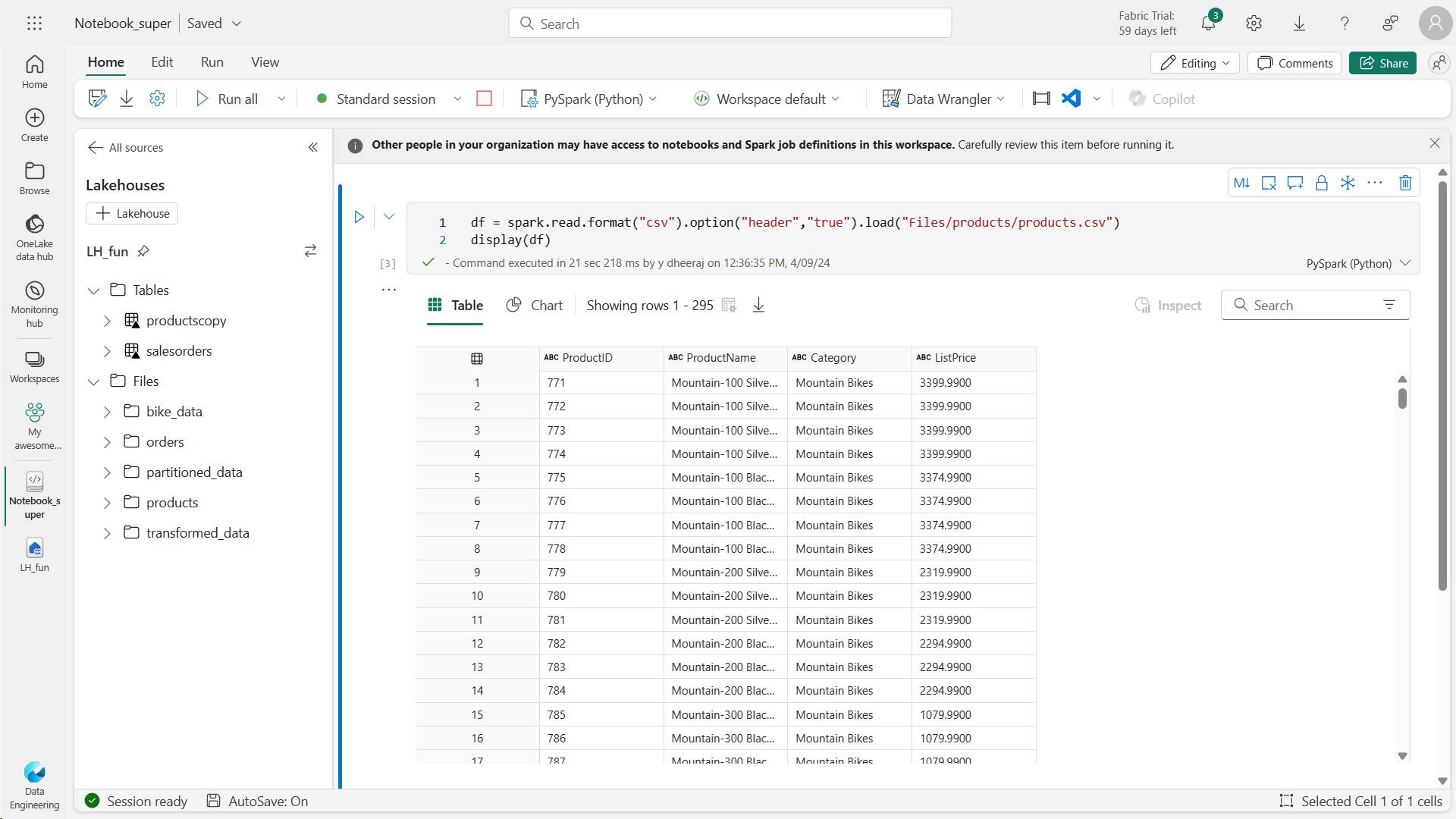
df = spark.read.format("csv").option("header","true").load("Files/products/products.csv")
# df now is a Spark DataFrame containing CSV data from "Files/products/products.csv".
display(df)
iv. Create delta tables
a. Create a managed table
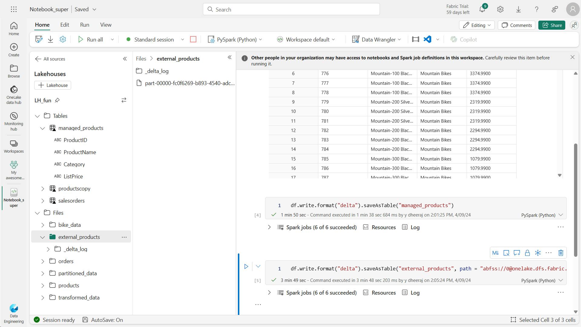
df.write.format("delta").saveAsTable("managed_products")
b. Create an external table
df.write.format("delta").saveAsTable("external_products", path="abfs_path/external_products")
c. Compare managed and external tables
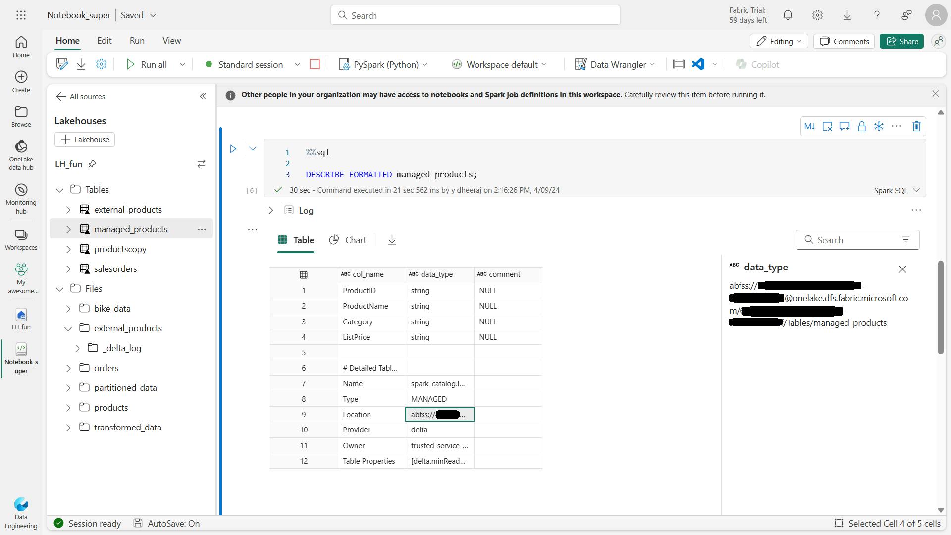
%%sql

DESCRIBE FORMATTED managed_products;
In the results, view the Location property for the table, which should be a path to the OneLake storage for the lakehouse ending with /Tables/managed_products (you may need to widen the Data type column to see the full path).
%%sql
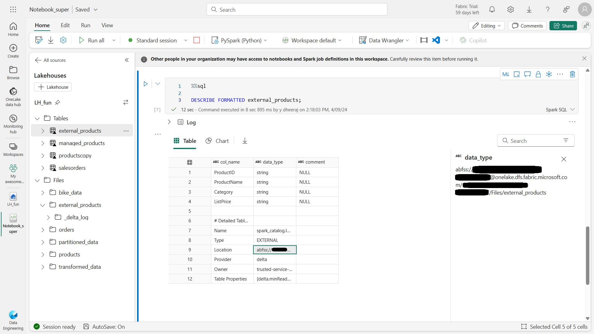
DESCRIBE FORMATTED external_products;
In the results, view the Location property for the table, which should be a path to the OneLake storage for the lakehouse ending with /Files/external_products (you may need to widen the Data type column to see the full path).
The files for managed table are stored in the Tables folder in the OneLake storage for the lakehouse. In this case, a folder named managed_products has been created to store the Parquet files and delta_log folder for the table you created.
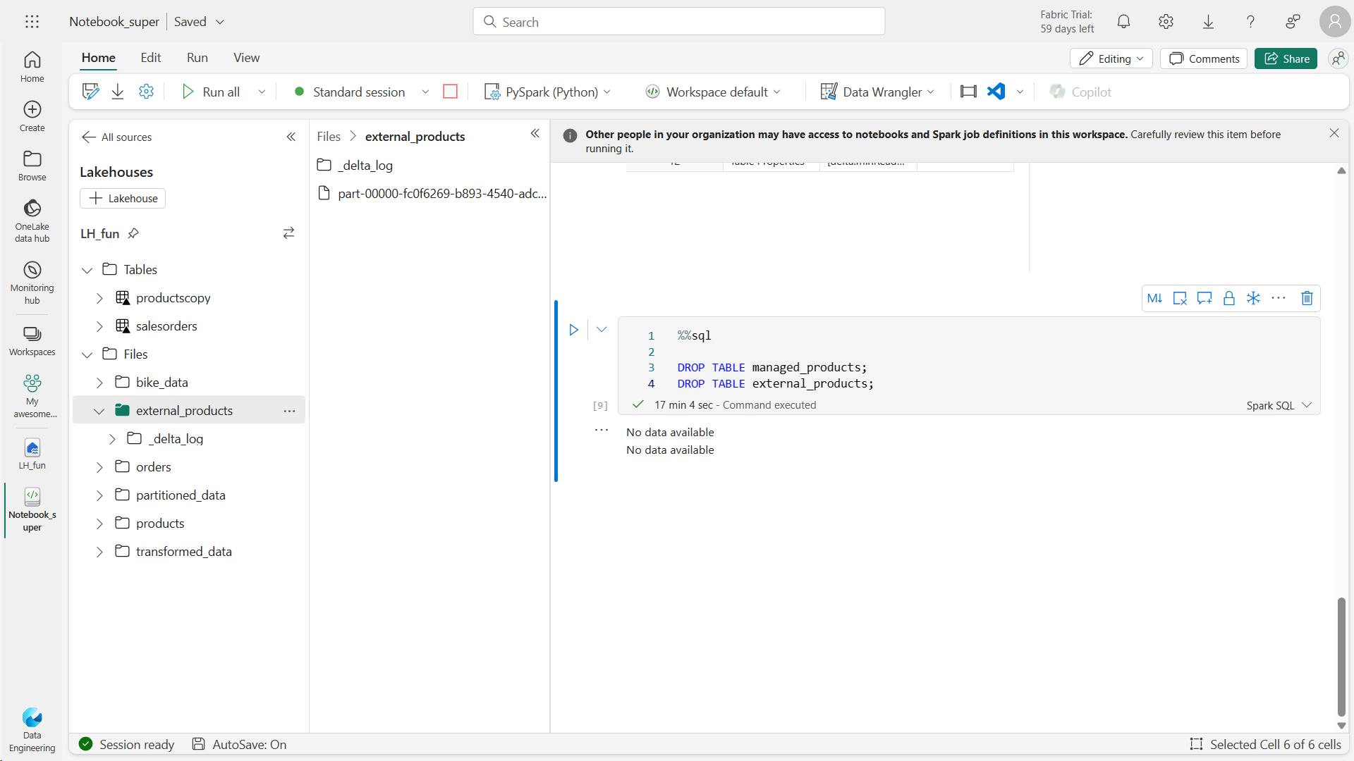
drop
%%sql

DROP TABLE managed_products;
DROP TABLE external_products;
d. Use SQL to create a table
%%sql

CREATE TABLE products
USING DELTA
LOCATION 'Files/external_products';
In the Lakehouse explorer pane, in the … menu for the Tables folder, select Refresh. Then expand the Tables node and verify that a new table named products is listed. Then expand the table to verify that its schema matches the original dataframe that was saved in the external_products folder.
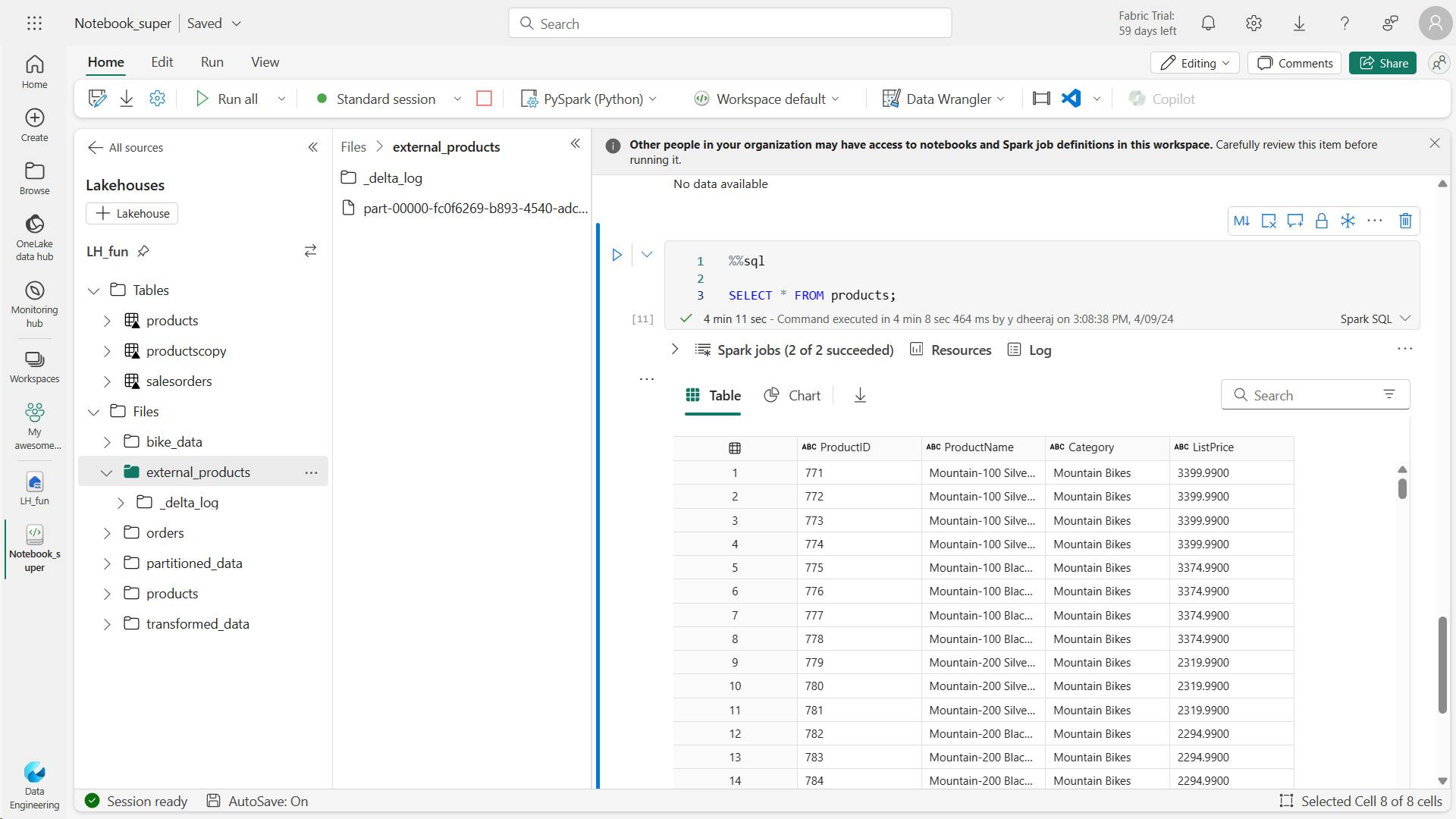
%%sql

SELECT * FROM products;
v. Explore table versioning
%%sql

UPDATE products
SET ListPrice = ListPrice * 0.9
WHERE Category = 'Mountain Bikes';
show the history of transactions recorded for the table
%%sql

DESCRIBE HISTORY products;
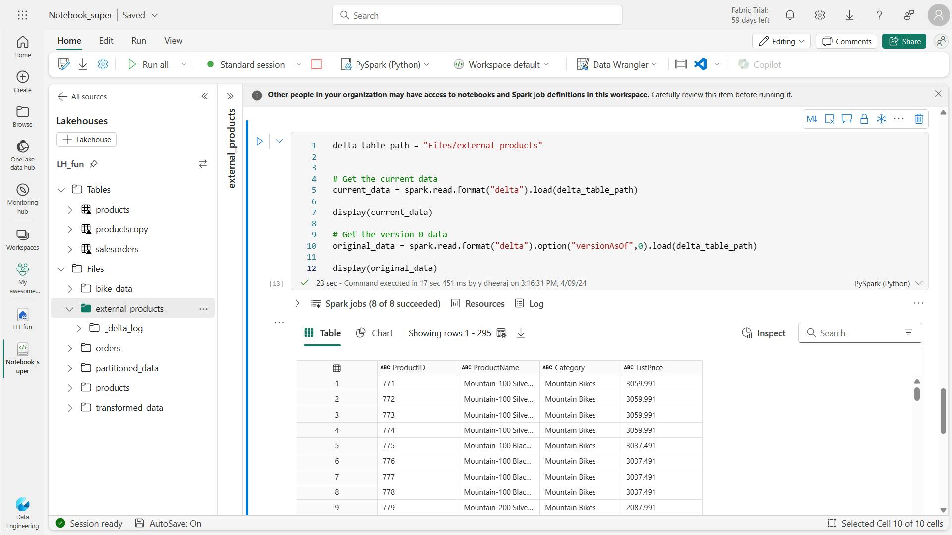
veversionAsOf
delta_table_path = 'Files/external_products'

# Get the current data
current_data = spark.read.format("delta").load(delta_table_path)
display(current_data)

# Get the version 0 data
original_data = spark.read.format("delta").option("versionAsOf", 0).load(delta_table_path)
display(original_data)
vi. Use delta tables for streaming data
Delta lake supports streaming data. Delta tables can be a sink or a source for data streams created using the Spark Structured Streaming API.
In this example, you’ll use a delta table as a sink for some streaming data in a simulated internet of things (IoT) scenario.
from notebookutils import mssparkutils
from pyspark.sql.types import *
from pyspark.sql.functions import *

# Create a folder
inputPath = 'Files/data/'
mssparkutils.fs.mkdirs(inputPath)

# Create a stream that reads data from the folder, using a JSON schema
jsonSchema = StructType([
StructField("device", StringType(), False),
StructField("status", StringType(), False)
])
iotstream = spark.readStream.schema(jsonSchema).option("maxFilesPerTrigger", 1).json(inputPath)

# Write some event data to the folder
device_data = '''{"device":"Dev1","status":"ok"}
{"device":"Dev1","status":"ok"}
{"device":"Dev1","status":"ok"}
{"device":"Dev2","status":"error"}
{"device":"Dev1","status":"ok"}
{"device":"Dev1","status":"error"}
{"device":"Dev2","status":"ok"}
{"device":"Dev2","status":"error"}
{"device":"Dev1","status":"ok"}'''
mssparkutils.fs.put(inputPath + "data.txt", device_data, True)
print("Source stream created...")
This code writes the streaming device data in delta format to a folder named iotdevicedata. Because the path for the folder location in the Tables folder, a table will automatically be created for it.
# Write the stream to a delta table
delta_stream_table_path = 'Tables/iotdevicedata'
checkpointpath = 'Files/delta/checkpoint'
deltastream = iotstream.writeStream.format("delta").option("checkpointLocation", checkpointpath).start(delta_stream_table_path)
print("Streaming to delta sink...")

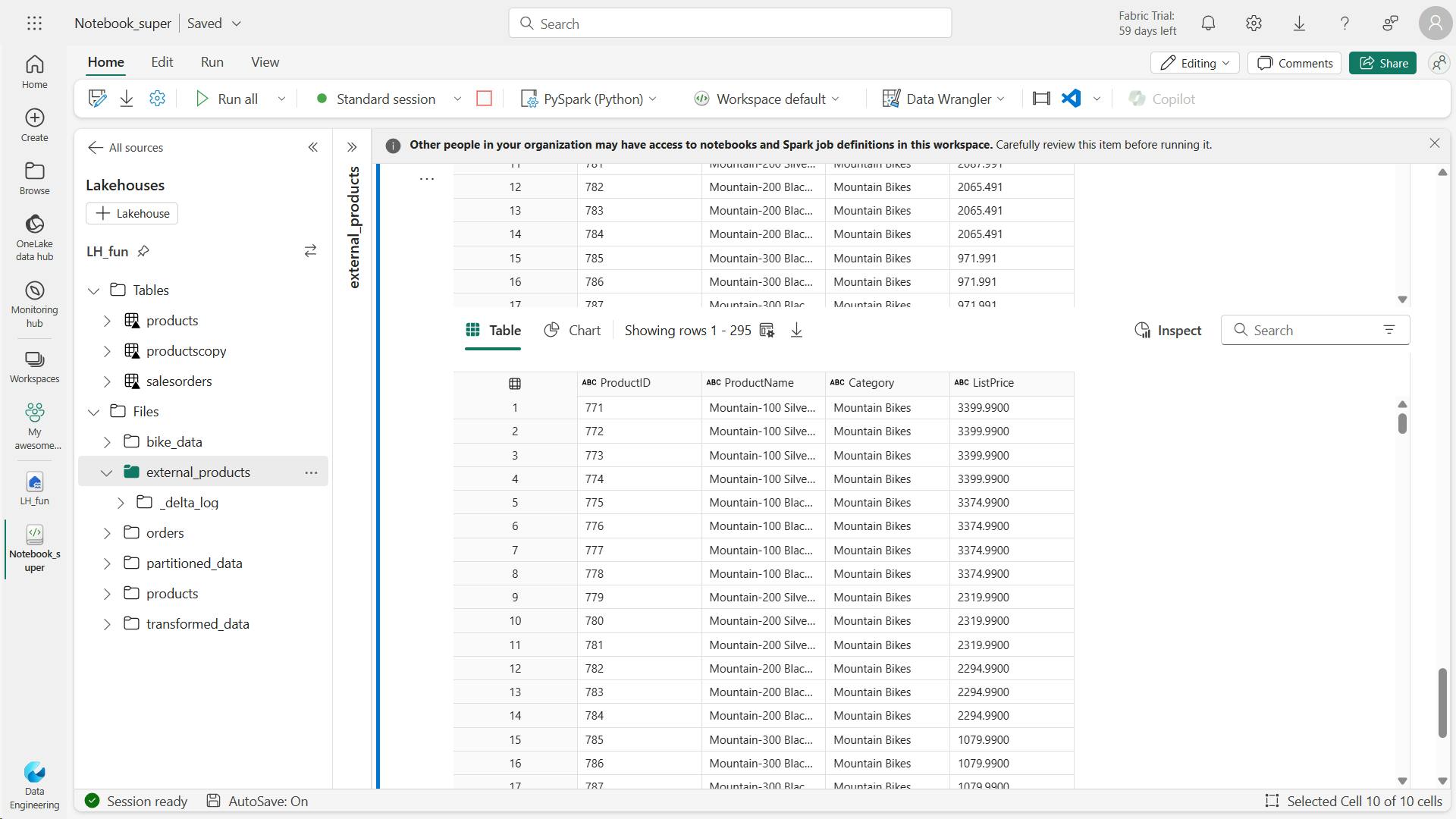
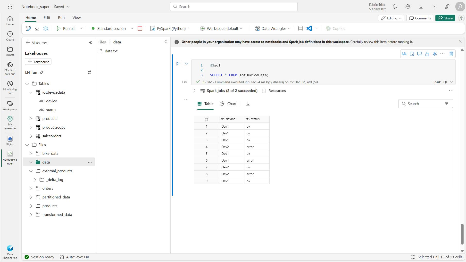
code queries the IotDeviceData table, which contains the device data from the streaming source.
%%sql

SELECT * FROM IotDeviceData;
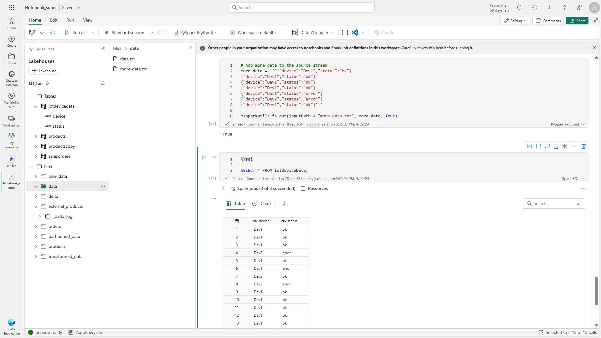
code writes more hypothetical device data to the streaming source.
# Add more data to the source stream
more_data = '''{"device":"Dev1","status":"ok"}
{"device":"Dev1","status":"ok"}
{"device":"Dev1","status":"ok"}
{"device":"Dev1","status":"ok"}
{"device":"Dev1","status":"error"}
{"device":"Dev2","status":"error"}
{"device":"Dev1","status":"ok"}'''

mssparkutils.fs.put(inputPath + "more-data.txt", more_data, True)
This code queries the IotDeviceData table again, which should now include the additional data that was added to the streaming source.
%%sql

SELECT * FROM IotDeviceData;
This code stops the stream.
deltastream.stop()
vii. Clean up resources
7. Knowledge check
Which of the following descriptions best fits Delta Lake?
A relational storage layer for Spark that supports tables based on Parquet files.
Delta Lake provides a relational storage layer in which you can create tables based on Parquet files in a data lake.
You've loaded a Spark dataframe with data, that you now want to use in a delta table. What format should you use to write the dataframe to storage?
Storing a dataframe in DELTA format creates parquet files for the data and the transaction log metadata necessary for Delta Lake tables.
You have a managed table based on a folder that contains data files in delta format. If you drop the table, what happens?
The life-cycle of the metadata and data for a managed table are the same.
8. Summary
Delta Lake is a technology that adds relational database semantics to Apache Spark. Tables in a Microsoft Fabric lakehouse are based on Delta Lake, enabling you to take advantage of many advanced features and techniques through the Delta Lake API.
Learning objectives
Delta Lake, Delta table in lakehouse
Managed table, External tables
Creating table metadata
dataframe to a new folder location in delta format
delta tables (or delta format files) to retrieve and modify data
history of a Managed & External table, you can use the DESCRIBE SQL command
retrieve version of the data by reading the delta file location into a dataframe using versionAsOf & timestampAsOf
Spark Structured Streaming API
delta table as a streaming source & sink.
Create a managed table & External tables
delta tables for streaming data
In this module, you'll learn how to:
Understand Delta Lake and delta tables in Microsoft Fabric
Create and manage delta tables using Spark
Use Spark to query and transform data in delta tables
Use delta tables with Spark structured streaming
V. Use Data Factory pipelines in Microsoft Fabric
Microsoft Fabric includes Data Factory capabilities, including the ability to create pipelines that orchestrate data ingestion and transformation tasks.
1. Introduction
Data pipelines define a sequence of activities that orchestrate an overall process, usually by extracting data from one or more sources and loading it into a destination; often transforming it along the way.
Pipelines are commonly used to automate extract, transform, and load (ETL) processes that ingest transactional data from operational data stores into an analytical data store, such as a lakehouse or data warehouse.
They use the same architecture of connected activities to define a process that can include multiple kinds of data processing tasks and control flow logic.
You can run pipelines interactively in the Microsoft Fabric user interface, or schedule them to run automatically.
2. Understand pipelines
Pipelines in Microsoft Fabric encapsulate a sequence of activities that perform data movement and processing tasks.
You can use a pipeline to define data transfer and transformation activities, and orchestrate these activities through control flow activities that manage branching, looping, and other typical processing logic.
The graphical pipeline canvas in the Fabric user interface enables you to build complex pipelines with minimal or no coding required.
i. Core pipeline concepts
a. Activities
Activities are the executable tasks in a pipeline. You can define a flow of activities by connecting them in a sequence. The outcome of a particular activity (success, failure, or completion) can be used to direct the flow to the next activity in the sequence.
There are two broad categories of activity in a pipeline.
1. Data transformation activities -
activities that encapsulate data transfer operations, including simple Copy Data activities that extract data from a source and load it to a destination, and more complex Data Flow activities that encapsulate dataflows (Gen2) that apply transformations to the data as it is transferred. Other data transformation activities include Notebook activities to run a Spark notebook, Stored procedure activities to run SQL code, Delete data activities to delete existing data, and others.
2. Control flow activities -
activities that you can use to implement loops, conditional branching, or manage variable and parameter values. The wide range of control flow activities enables you to implement complex pipeline logic to orchestrate data ingestion and transformation flow.
b Parameters
Pipelines can be parameterized, enabling you to provide specific values to be used each time a pipeline is run. For example, you might want to use a pipeline to save ingested data in a folder, but have the flexibility to specify a folder name each time the pipeline is run.
Using parameters increases the reusability of your pipelines, enabling you to create flexible data ingestion and transformation processes.
c Pipeline runs
Each time a pipeline is executed, a data pipeline run is initiated. Runs can be initiated on-demand in the Fabric user interface or scheduled to start at a specific frequency. Use the unique run ID to review run details to confirm they completed successfully and investigate the specific settings used for each execution.
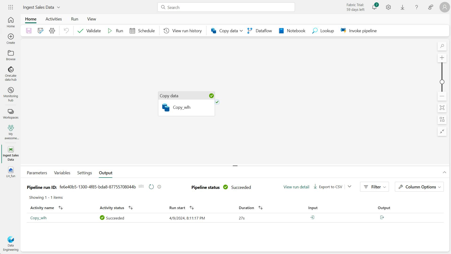
3. Use the Copy Data activity
Many pipelines consist of a single Copy Data activity that is used to ingest data from an external source into a lakehouse file or table.
You can also combine the Copy Data activity with other activities to create a repeatable data ingestion process - for example by using a Delete data activity to remove existing data, a Copy Data activity to replace the deleted data with a file containing data from an external source, and a Notebook activity to run Spark code that transforms the data in the file and loads it into a table.
i. The Copy Data tool
ii. Copy Data activity settings
iii. When to use the Copy Data activity
Use the Copy Data activity when you need to copy data directly between a supported source and destination without applying any transformations, or when you want to import the raw data and apply transformations in later pipeline activities.
If you need to apply transformations to the data as it is ingested, or merge data from multiple sources, consider using a Data Flow activity to run a dataflow (Gen2). You can use the Power Query user interface to define a dataflow (Gen2) that includes multiple transformation steps, and include it in a pipeline.
4. Use pipeline templates
You can define pipelines from any combination of activities you choose, enabling to create custom data ingestion and transformation processes to meet your specific needs. However, there are many common pipeline scenarios for which Microsoft Fabric includes predefined pipeline templates that you can use and customize as required.
5. Run and monitor pipelines
When you have completed a pipeline, you can use the Validate option to check that is configuration is valid, and then either run it interactively or specify a schedule.
6. Exercise - Ingest data with a pipeline
i. Create a workspace
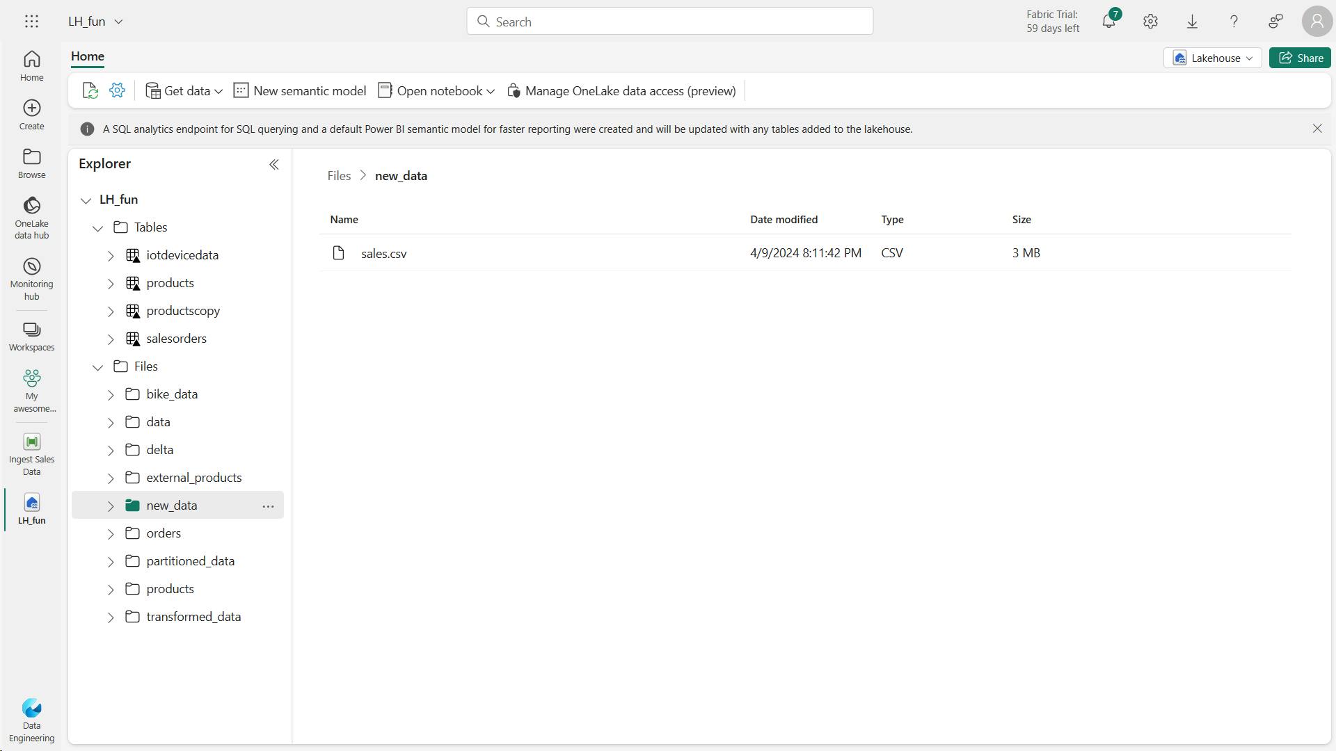
ii. Create a lakehouse
new_data
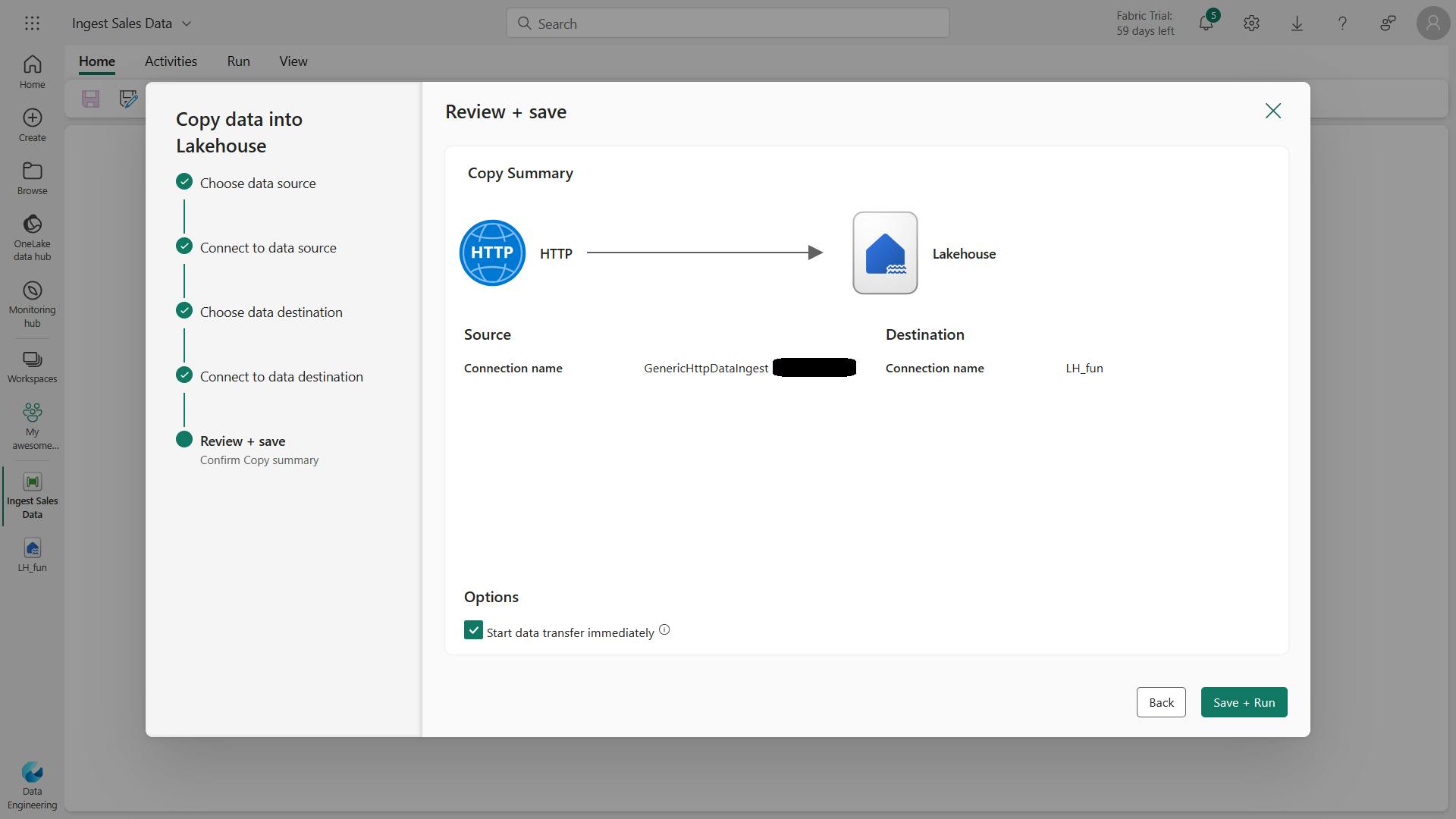
iii. Create a pipeline
Ingest Sales Data
In LH:
iv. Create a notebook
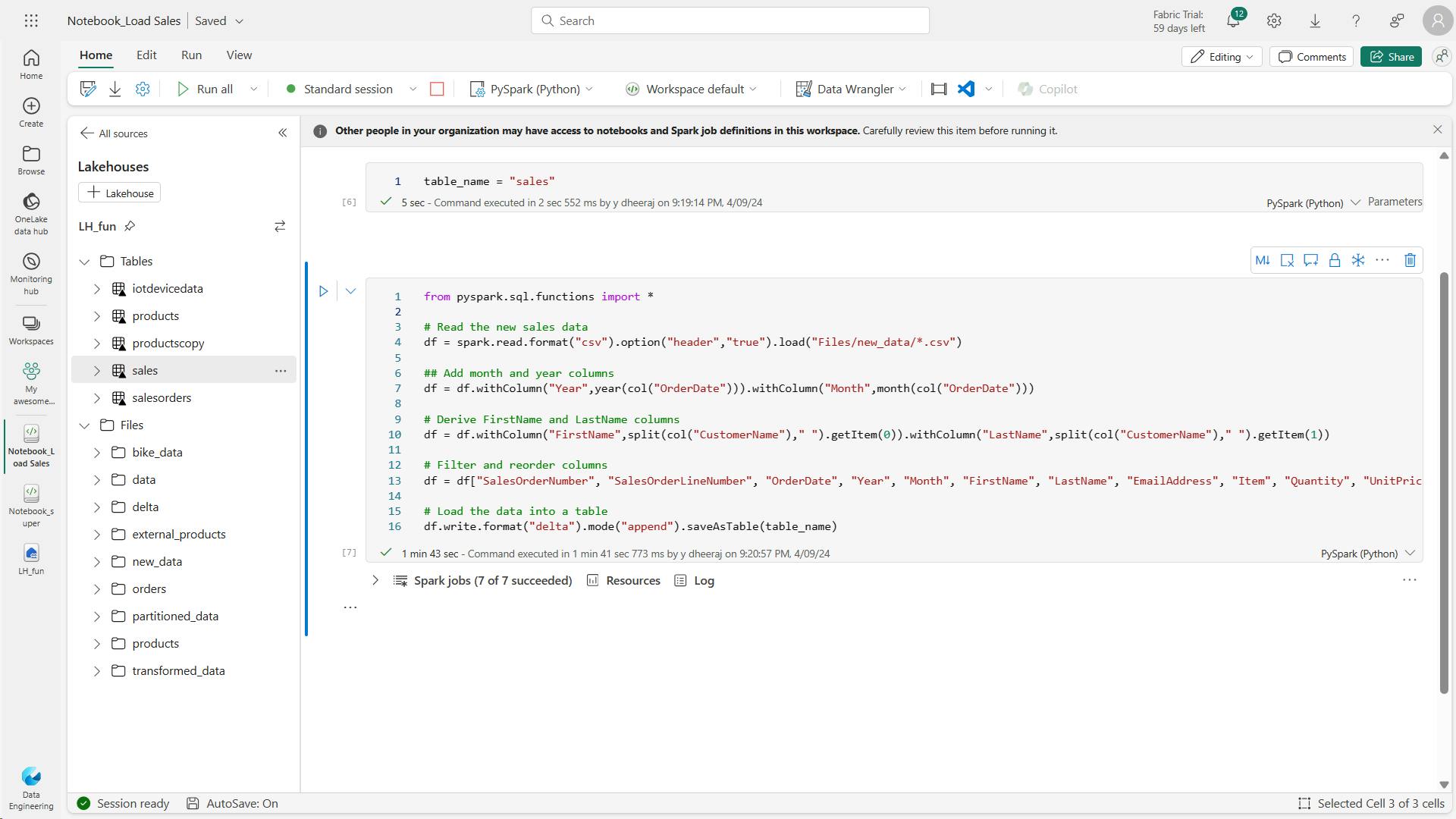
In the … menu for the cell (at its top-right) select Toggle parameter cell. This configures the cell so that the variables declared in it are treated as parameters when running the notebook from a pipeline.
This code loads the data from the sales.csv file that was ingested by the Copy Data activity, applies some transformation logic, and saves the transformed data as a table - appending the data if the table already exists.
from spark.sql.functions import *

# Read the new sales data
df = spark.read.format("csv").option("header","true").load("Files/new_data/*.csv")

## Add month and year columns
df = df.withColumn("Year",year(col("OrderDate"))).withColumn("Month",month(col("OrderDate")))

# Derive FirstName and LastName columns
df = df.withColumn("FirstName",split(col("CustomerName")," ").getItem(0)).withColumn("LastName",split(col("CustomerName")," ").getItem(1))

# Filter and reorder columns
df = df["SalesOrderNumber", "SalesOrderLineNumber", "OrderDate", "Year", "Month", "FirstName", "LastName", "EmailAddress", "Item", "Quantity", "UnitPrice", "TaxAmount"]

# Load the data into a table
df.write.format("delta").mode("append").saveAsTable("table_name")
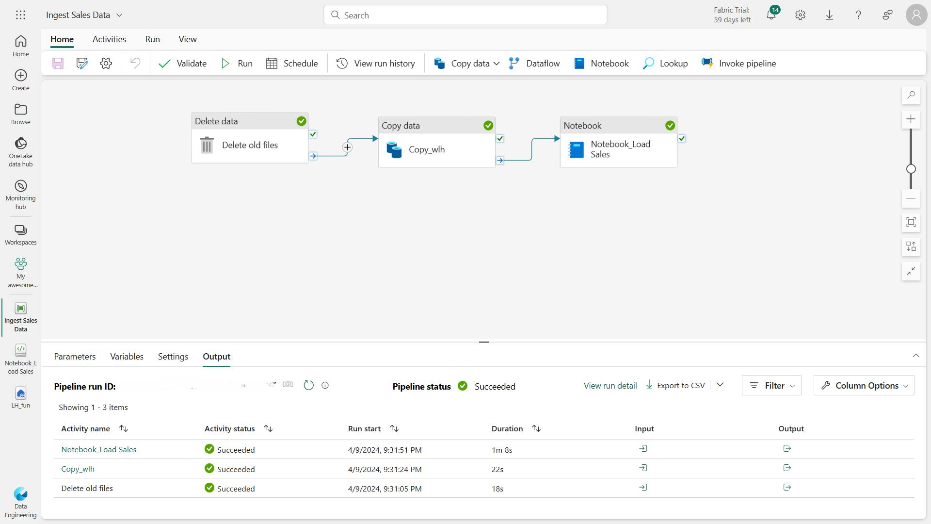
v. Modify the pipeline
Now that you’ve implemented a notebook to transform data and load it into a table, you can incorporate the notebook into a pipeline to create a reusable ETL process.
The table_name parameter will be passed to the notebook and override the default value assigned to the table_name variable in the parameters cell.
In this exercise, you implemented a data ingestion solution that uses a pipeline to copy data to your lakehouse from an external source, and then uses a Spark notebook to transform the data and load it into a table.
vi. Clean up resources
7. Knowledge check
What is a data pipeline?
A sequence of activities to orchestrate a data ingestion or transformation process
A pipeline consists of activities to ingest and transform data.
You want to use a pipeline to copy data to a folder with a specified name for each run. What should you do?
Add a parameter to the pipeline and use it to specify the folder name for each run
Using a parameter enables greater flexibility for your pipeline.
You have previously run a pipeline containing multiple activities. What's the best way to check how long each individual activity took to complete?
View the run details in the run history.
The run history details show the time taken for each activity - optionally as a Gantt chart.
8. Summary
With Microsoft Fabric, you can create pipelines that encapsulate complex data ingestion and transformation processes. Pipelines provide an effective way to orchestrate data processing tasks that can be run on-demand or at scheduled intervals.
Learning objectives
In this module, you'll learn how to:
Describe pipeline capabilities in Microsoft Fabric
Use the Copy Data activity in a pipeline
Create pipelines based on predefined templates
Run and monitor pipelines
implemented a data ingestion solution that uses a pipeline to copy data to lakehouse from an external source, and then a Spark notebook to transform the data and load it into a table.
VI. Ingest Data with Dataflows Gen2 in Microsoft Fabric
Data ingestion is crucial in analytics.
Microsoft Fabric's Data Factory offers Dataflows for visually creating multi-step data ingestion and transformation using Power Query Online.
1. Introduction
Dataflows Gen2 are used to ingest and transform data from multiple sources, and then land the cleansed data to another destination.
They can be incorporated into data pipelines for additional data movement, and used as a data source in Power BI.
2. Understand Dataflows Gen2 in Microsoft Fabric
By using Dataflows Gen2, you can connect to the various data sources, and then prep and transform the data.
To allow access, you can land the data directly into your Lakehouse or use a data pipeline for other destinations.
i. What is a dataflow?
Dataflows are a type of cloud-based ETL (Extract, Transform, Load) tool for building and executing scalable data transformation processes.
Dataflows Gen2 allow you to extract data from various sources, transform it using a wide range of transformation operations, and load it into a destination. Using Power Query Online also allows for a visual interface to perform these tasks.
Fundamentally, a dataflow includes all of the transformations to reduce data prep time and then can be loaded into a new table, included in a Data Pipeline, or used as a data source by data analysts.
ii. How to use Dataflows Gen2
Traditionally, data engineers spend significant time extracting, transforming, and loading data into a consumable format for downstream analytics.
The goal of Dataflows Gen2 is to provide an easy, reusable way to perform ETL tasks using Power Query Online.
If you only choose to use a Data Pipeline, you copy data, then use your preferred coding language to extract, transform, and load the data.
Alternatively, you can create a Dataflow Gen2 first to extract and transform the data. You can also load the data into a Lakehouse, and other destinations.
To perform other tasks or load data to a different destination after transformation, create a Data Pipeline and add the Dataflow Gen2 activity to your orchestration.
Another option might be to use a Data Pipeline and Dataflow Gen2 for ELT (Extract, Load, Transform) process.
For this order, you'd use a Pipeline to extract and load the data into your preferred destination, such as the Lakehouse.
Then you'd create a Dataflow Gen2 to connect to Lakehouse data to cleanse and transform data. In this case, you'd offer the Dataflow as a curated semantic model for data analysts to develop reports.
Dataflows allow you to promote reusable ETL logic that prevents the need to create more connections to your data source.
Dataflows offer a wide variety of transformations, and can be run manually, on a refresh schedule, or as part of a Data Pipeline orchestration.
iii Benefits and limitations
There's more than one way to ETL or ELT data in Microsoft Fabric. Consider the benefits and limitations for using Dataflows Gen2.
Benefits:
Extend data with consistent data, such as a standard date dimension table.
Allow self-service users access to a subset of data warehouse separately.
Optimize performance with dataflows, which enable extracting data once for reuse, reducing data refresh time for slower sources.
Simplify data source complexity by only exposing dataflows to larger analyst groups.
Ensure consistency and quality of data by enabling users to clean and transform data before loading it to a destination.
Simplify data integration by providing a low-code interface that ingests data from various sources.
Limitations:
Not a replacement for a data warehouse.
Row-level security isn't supported.
Fabric capacity workspace is required.
3. Explore Dataflows Gen2 in Microsoft Fabric
In Microsoft Fabric, you can create a Dataflow Gen2 in the Data Factory workload or Power BI workspace, or directly in the lakehouse.
Since our scenario is focused on data ingestion, let's look at the Data Factory workload experience.
Dataflows Gen2 use Power Query Online to visualize transformations.
i. Power Query ribbon
ii. Queries pane
iii. Diagram view
iv. Data Preview pane
v. Query Settings pane
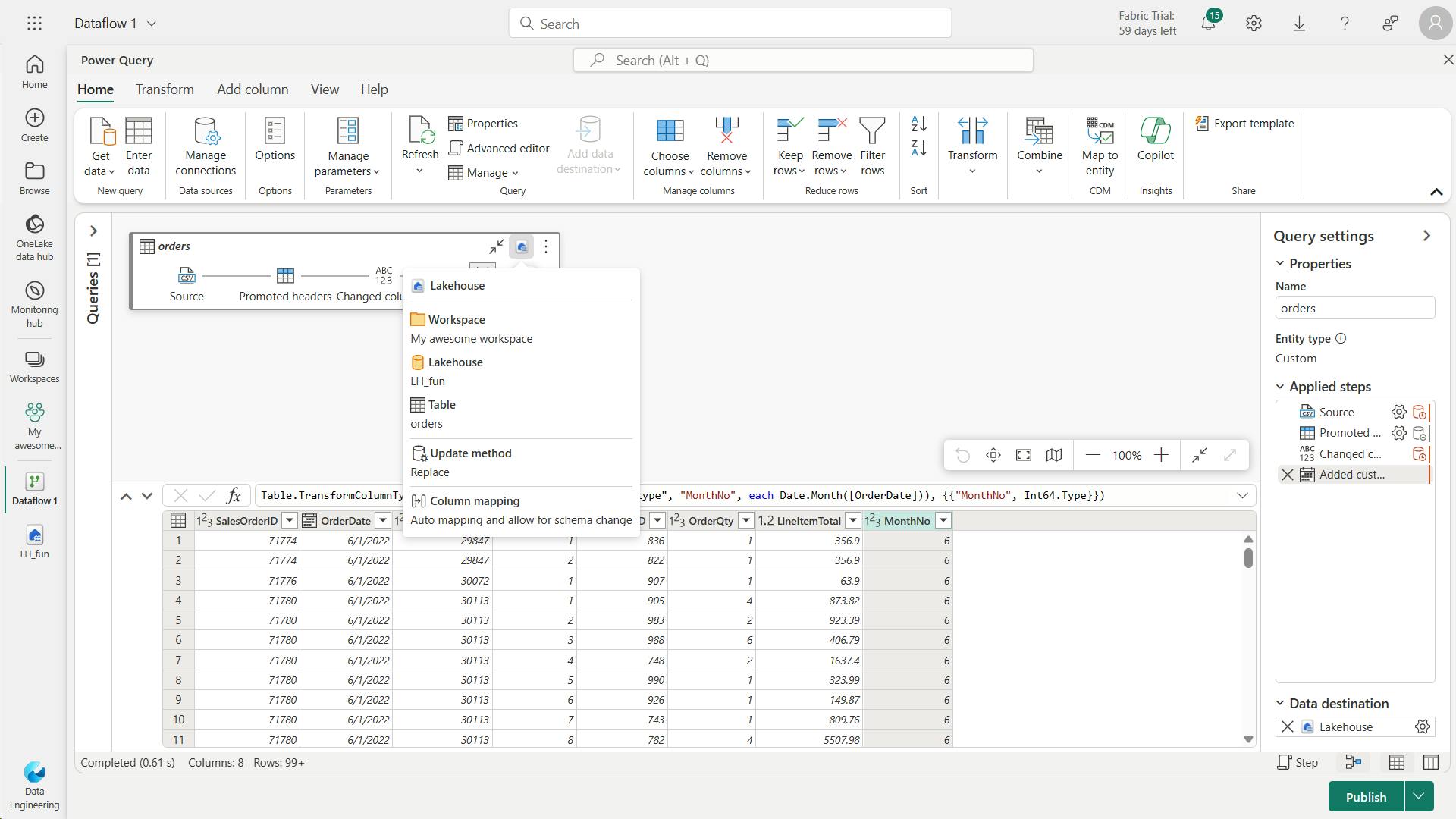
In the Query settings pane, you can see a Data Destination field where you can set the Lakehouse as your destination
4. Integrate Dataflows Gen2 and Pipelines in Microsoft Fabric
The combination of dataflows and pipelines is useful when you need to perform additional operations on the transformed data.
Data pipelines are easily created in the Data Factory and Data Engineering workloads. Pipelines are a common concept in data engineering and offer a wide variety of activities to orchestrate. Some common activities include:
Copy data
Incorporate Dataflow
Add Notebook
Get metadata
Execute a script or stored procedure
Pipelines provide a visual way to complete activities in a specific order. You can use a dataflow for data ingestion and transformation, and landing into a Lakehouse using dataflows.
Then incorporate the dataflow into a pipeline to orchestrate extra activities, like execute scripts or stored procedures after the dataflow has completed.
5. Exercise - Create and use a Dataflow Gen2 in Microsoft Fabric
In this module, we walked through a scenario where both data engineers and data analysts have a need to prepare data for consumption and expand semantic models.
We identified Dataflows Gen2 as the best solution for the data transformation steps.
In this exercise, you create and use a Dataflow Gen2 to ingest transformed data into a Lakehouse.
In Microsoft Fabric, Dataflows (Gen2) connect to various data sources and perform transformations in Power Query Online. They can then be used in Data Pipelines to ingest data into a lakehouse or other analytical store, or to define a dataset for a Power BI report.
This lab is designed to introduce the different elements of Dataflows (Gen2), and not create a complex solution that may exist in an enterprise.
i. Create a workspace
ii. Create a lakehouse
iii. Create a Dataflow (Gen2) to ingest data
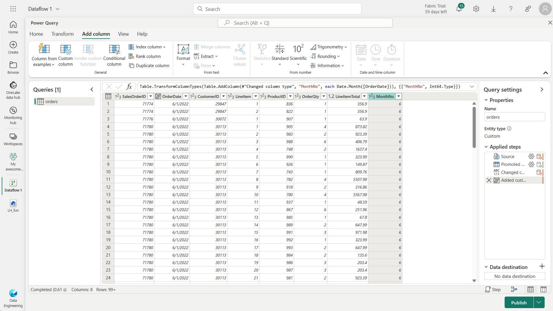
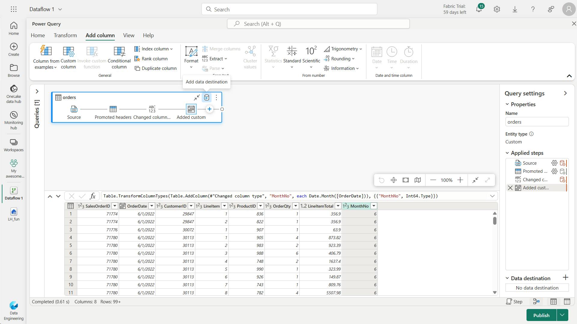
iv. Add data destination for Dataflow
v. Add a dataflow to a pipeline
You can include a dataflow as an activity in a pipeline.
Pipelines are used to orchestrate data ingestion and processing activities, enabling you to combine dataflows with other kinds of operation in a single, scheduled process.
Pipelines can be created in a few different experiences, including Data Factory experience.


vi. Clean up resources
6. Knowledge check
What is a Dataflow Gen2?
A way to import and transform data with Power Query Online.
Dataflow Gen2 allows you to get and transform data, then optionally ingest to a Lakehouse.
Which workload experience lets you create a Dataflow Gen2?
Data Factory.
Data Factory and Power BI workloads allow Dataflow Gen2 creation.
You need to connect to and transform data to be loaded into a Fabric Lakehouse and also loaded into a KQL Database for Real-time Analytics. You aren't comfortable using Spark notebooks, so decide to use Dataflows Gen2. How would you complete this task?
Connect to Data Factory workload > Create Dataflows Gen2 to transform data > Create Data pipeline to include your dataflow and then land data to a KQL Database.
These are the high-level steps to accomplish your task.
7. Summary
With Microsoft Fabric, you can create Dataflows Gen2 to perform data integration for your Lakehouse, and optionally include the dataflow in a Data Pipeline as well.
In this module, you learned about Dataflows Gen2 and how to use them as part of your data integration process.
Power Query Online offers a visual interface to perform complex data transformations without writing any code.
Learning objectives
In this module, you'll learn how to:
Describe Dataflow Gen2 capabilities in Microsoft Fabric
Create Dataflow Gen2 solutions to ingest and transform data
Include a Dataflow Gen2 in a pipeline
VII. Ingest data with Spark and Microsoft Fabric notebooks
Discover how to use Apache Spark and Python for data ingestion into a Microsoft Fabric lakehouse. Fabric notebooks provide a scalable and systematic solution.
1. Introduction
Fabric notebooks offer the flexibility to extract, load, and transform external data into your lakehouse, adapting to your workflow.
Fabric notebooks are the best choice if you:
Handle large external data Need complex transformations.
By the end of this module, you'll be able to use Spark and Fabric notebooks to ingest external data into your lakehouse. You'll also learn fundamental transformations and optimization techniques for a more efficient ETL process.
2. Connect to data with Spark
First, let's discuss what Fabric notebooks offer over the other ingestion options.
Unlike manual uploads, notebooks provide automation, ensuring a smooth and systematic approach.
Dataflows offer a UI experience; however, they aren't as performant with large semantic models.
Pipelines allow you to orchestrate the Copy Data, and may require dataflows or notebooks for transformations.
Therefore, notebooks provide a comprehensive, automated solution for ingestion and transformation.
i. Explore Fabric notebooks
By default, Fabric notebooks use PySpark, which uses the Spark engine to allow a multi-threaded, distributed transaction for speedy processes.
You can use Html, Spark (Scala), Spark SQL, and SparkR (R) as well, however they may not have the full benefit of the distributed system.
ii. Connect to external sources
connecting to Azure blob storage with Spark:
The PySpark code defines the parameters and constructs the connection path, then reads the data into a DataFrame and shows the data in the DataFrame.
# Azure Blob Storage access info
blob_account_name = "azureopendatastorage"
blob_container_name = "nyctlc"
blob_relative_path = "yellow"
blob_sas_token = "sv=2022-11-02&ss=bfqt&srt=c&sp=rwdlacupiytfx&se=2023-09-08T23:50:02Z&st=2023-09-08T15:50:02Z&spr=https&sig=abcdefg123456"

# Construct the path for connection
wasbs_path = f'wasbs://{blob_container_name}@{blob_account_name}.blob.core.windows.net/{blob_relative_path}?{blob_sas_token}'

# Read parquet data from Azure Blob Storage path
blob_df = spark.read.parquet(wasbs_path)

# Show the Azure Blob DataFrame
blob_df.show()
iii. Configure alternate authentication
The previous example connects to the source and reads the data into a DataFrame.
Depending on your source, you may need a different authentication type, such as Service Principal, OAuth, etc.
Here's an example connecting to an Azure SQL Database with a Service Principal:
# Placeholders for Azure SQL Database connection info
server_name = "your_server_name.database.windows.net"
port_number = 1433  # Default port number for SQL Server
database_name = "your_database_name"
table_name = "YourTableName" # Database table
client_id = "YOUR_CLIENT_ID"  # Service principal client ID
client_secret = "YOUR_CLIENT_SECRET"  # Service principal client secret
tenant_id = "YOUR_TENANT_ID"  # Azure Active Directory tenant ID


# Build the Azure SQL Database JDBC URL with Service Principal (Active Directory Integrated)
jdbc_url = f"jdbc:sqlserver://{server_name}:{port_number};database={database_name};encrypt=true;trustServerCertificate=false;hostNameInCertificate=*.database.windows.net;loginTimeout=30;Authentication=ActiveDirectoryIntegrated"

# Properties for the JDBC connection
properties = {
    "user": client_id,
    "password": client_secret,
    "driver": "com.microsoft.sqlserver.jdbc.SQLServerDriver",
    "tenantId": tenant_id
}

# Read entire table from Azure SQL Database using AAD Integrated authentication
sql_df = spark.read.jdbc(url=jdbc_url, table=table_name, properties=properties)

# Show the Azure SQL DataFrame
sql_df.show()
3. Write data into a lakehouse
Now that we've connected to data, we need to save it into the lakehouse. You can either save as a file or load as a Delta table.
iv. Write to a file
Lakehouses support structured, semi-structured, and unstructured files.
Load as a parquet file or Delta table to take advantage of the Spark engine.
a. Write DataFrame to Parquet file format
# Write DataFrame to Parquet file format
parquet_output_path = "your_folder/your_file_name"
df.write.mode("overwrite").parquet(parquet_output_path)
print(f"DataFrame has been written to Parquet file: {parquet_output_path}")
b. Write DataFrame to Delta table
# Write DataFrame to Delta table
delta_table_name = "your_delta_table_name"
df.write.format("delta").mode("overwrite").saveAsTable(delta_table_name)
print(f"DataFrame has been written to Delta table: {delta_table_name}")
OneLake supports a wide variety of file formats, including many formats that are commonly used in Spark code - such as delimited text, JSON, Parquet, Avro, ORC, and others.
In most cases, Parquet is the preferred format because of its optimized columnar storage structure and efficient compression capabilities. Parquet is also the base format on which Delta tables in a lakehouse are based.
v. Write to a Delta table
Delta tables are one of the key features of Fabric lakehouses. Easily ingest and load your external data into a Delta table via notebooks.
# Use format and save to load as a Delta table
table_name = "nyctaxi_raw"
filtered_df.write.mode("overwrite").format("delta").save(f"Tables/{table_name}")

# Confirm load as Delta table
print(f"Spark DataFrame saved to Delta table: {table_name}")
vi. Optimize Delta table writes
Fabric notebooks easily scale for large data, therefore read and write optimization is key.
Consider these optimization functions for even more performant data ingestion.
a. V-Order
enables faster and more efficient reads by various compute engines, such as Power BI, SQL, and Spark.V-order applies special sorting, distribution, encoding, and compression on parquet files at write-time.
# Enable V-Order
spark.conf.set("spark.sql.parquet.vorder.enabled", "true")
b. Optimize write
improves the performance and reliability by reducing the number of files written and increasing their size. It's useful for scenarios where the Delta tables have suboptimal or nonstandard file sizes, or where the extra write latency is tolerable.
# Enable automatic Delta optimized write
spark.conf.set("spark.microsoft.delta.optimizeWrite.enabled", "true")
4. Consider uses for ingested data
You've now ingested raw data in the Fabric lakehouse, also known as the bronze layer of a Medallion architecture.
Before moving to the transformation and modeling steps, consider where to transform and how users interact with the data.
i. Transform for different users
When you load data, it's a good idea to do some basic cleaning like removing duplicates, handling errors, converting null values, and getting rid of empty entries to ensure data quality and consistency.
Also thinking about the different people who use the data is crucial.
Data scientists usually prefer fewer changes so they can explore wide tables. They would likely want access to the raw ingested data. Fabric's Data Wrangler then let's them explore the data and generate transformation code for their specific needs.
Whereas Power BI data analysts may require more transformation and modeling before they can use the data. While Power BI can transform data, starting with well-prepared data allows analysts to develop reports and insights more efficiently.
5. Exercise - Ingest data with Spark and Microsoft Fabric notebooks
In this lab, you'll create a Microsoft Fabric notebook and use PySpark to connect to an Azure Blob Storage path, then load the data into a lakehouse using write optimizations.
For this experience, you’ll build the code across multiple notebook code cells, which may not reflect how you will do it in your environment; however, it can be useful for debugging.
Because you’re also working with a sample dataset, the optimization doesn’t reflect what you may see in production at scale; however, you can still see improvement and when every millisecond counts, optimization is key.
i. Create a workspace
ii. Create workspace and lakehouse destination
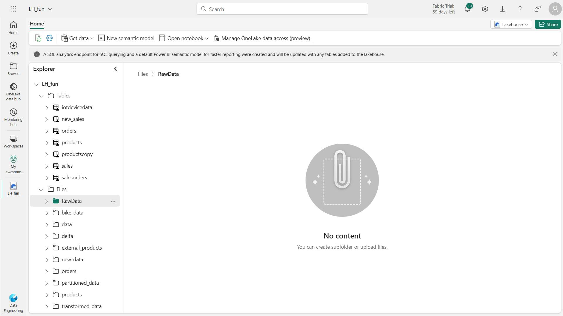
iii. Create a Fabric notebook and load external data
Insert the following code into the code cell, which will:
Declare parameters for connection string
Build the connection string
Read data into a DataFrame
a. Azure Blob Storage connection string:
 # Azure Blob Storage access info
 blob_account_name = "....."
 blob_container_name = "......."
 blob_relative_path = "......"

 # Construct connection path
 wasbs_path = f'wasbs://{blob_container_name}@{blob_account_name}.blob.core.windows.net/{blob_relative_path}'
 print(wasbs_path)

 # Read parquet data from Azure Blob Storage path
 blob_df = spark.read.parquet(wasbs_path)
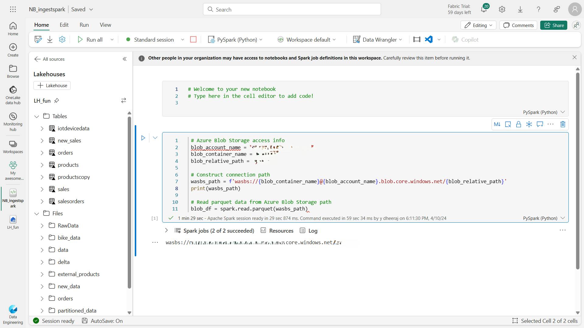
b. To write the data to a file, you now need that ABFS Path for your RawData folder.
# Declare file name
file_name = "yellow_taxi"

# Construct destination path
output_parquet_path = f"**InsertABFSPathHere**/{file_name}"
print(output_parquet_path)

# Load the first 1000 rows as a Parquet file
blob_df.limit(1000).write.mode("overwrite").parquet(output_parquet_path)
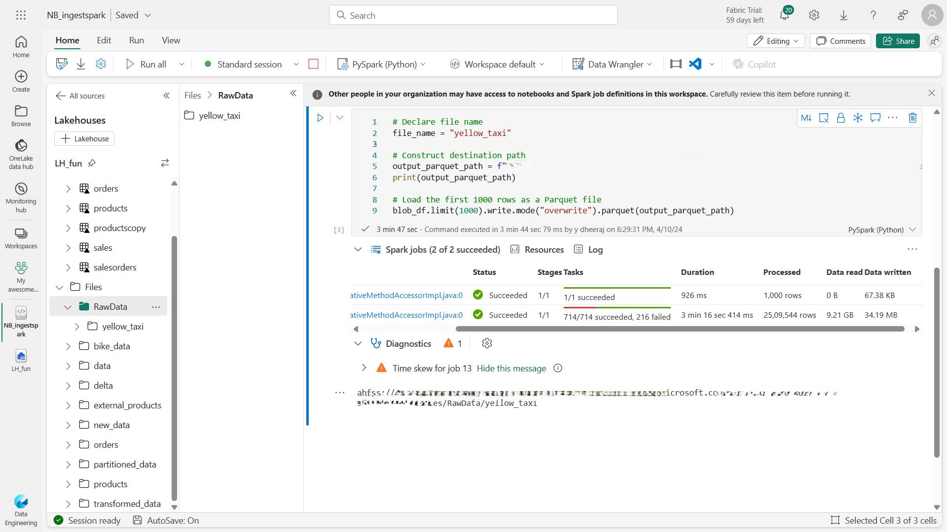
iv. Transform and load data to a Delta table
Likely, your data ingestion task doesn’t end with only loading a file.
Delta tables in a lakehouse allows scalable, flexible querying and storage, so we’ll create one as well.
This will add a timestamp column dataload_datetime to log when the data was loaded to a Delta table
Filter NULL values in storeAndFwdFlag
Load filtered data into a Delta table
Display a single row for validation
 from pyspark.sql.functions import col, to_timestamp, current_timestamp, year, month

 # Read the parquet data from the specified path
 raw_df = spark.read.parquet(output_parquet_path)

 # Add dataload_datetime column with current timestamp
 filtered_df = raw_df.withColumn("dataload_datetime", current_timestamp())

 # Filter columns to exclude any NULL values in storeAndFwdFlag
 filtered_df = filtered_df.filter(raw_df["storeAndFwdFlag"].isNotNull())

 # Load the filtered data into a Delta table
 table_name = "yellow_taxi"  # Replace with your desired table name
 filtered_df.write.format("delta").mode("append").saveAsTable(table_name)

 # Display results
 display(filtered_df.limit(1))
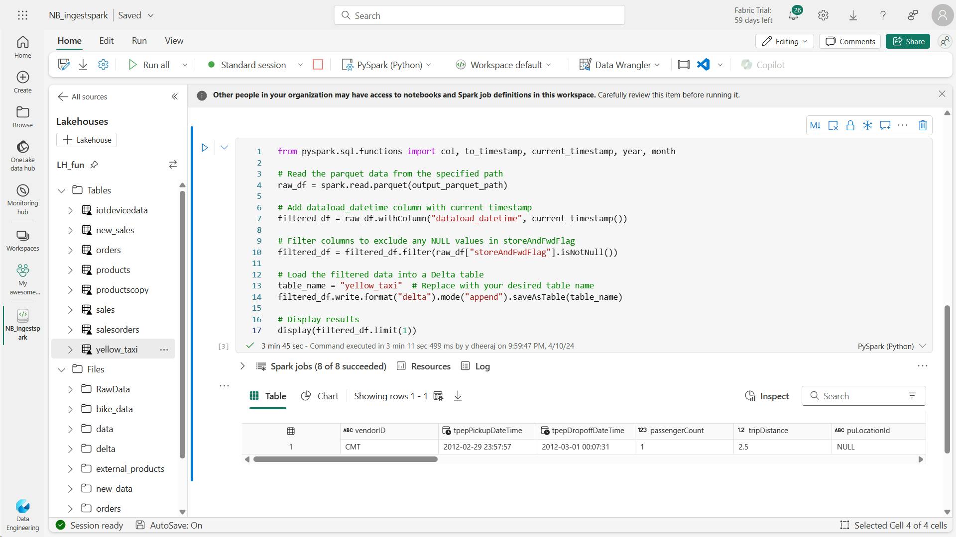
v. Optimize Delta table writes
You’re probably using big data in your organization and that’s why you chose Fabric notebooks for data ingestion, so let’s also cover how to optimize the ingestion and reads for your data. First, we’ll repeat the steps to transform and write to a Delta table with write optimizations included.
 from pyspark.sql.functions import col, to_timestamp, current_timestamp, year, month

 # Read the parquet data from the specified path
 raw_df = spark.read.parquet(output_parquet_path)

 # Add dataload_datetime column with current timestamp
 opt_df = raw_df.withColumn("dataload_datetime", current_timestamp())

 # Filter columns to exclude any NULL values in storeAndFwdFlag
 opt_df = opt_df.filter(opt_df["storeAndFwdFlag"].isNotNull())

 # Enable V-Order
 spark.conf.set("spark.sql.parquet.vorder.enabled", "true")

 # Enable automatic Delta optimized write
 spark.conf.set("spark.microsoft.delta.optimizeWrite.enabled", "true")

 # Load the filtered data into a Delta table
 table_name = "yellow_taxi_opt"  # New table name
 opt_df.write.format("delta").mode("append").saveAsTable(table_name)

 # Display results
 display(opt_df.limit(1))
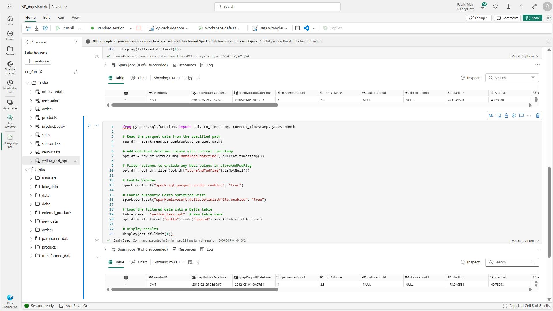
Now, take note of the run times for both code blocks. Your times will vary, but you can see a clear performance boost with the optimized code.
vi. Analyze Delta table data with SQL queries
 # Load table into df
 delta_table_name = "yellow_taxi"
 table_df = spark.read.format("delta").table(delta_table_name)

 # Create temp SQL table
 table_df.createOrReplaceTempView("yellow_taxi_temp")

 # SQL Query
 table_df = spark.sql('SELECT * FROM yellow_taxi_temp')

 # Display 10 results
 display(table_df.limit(10))
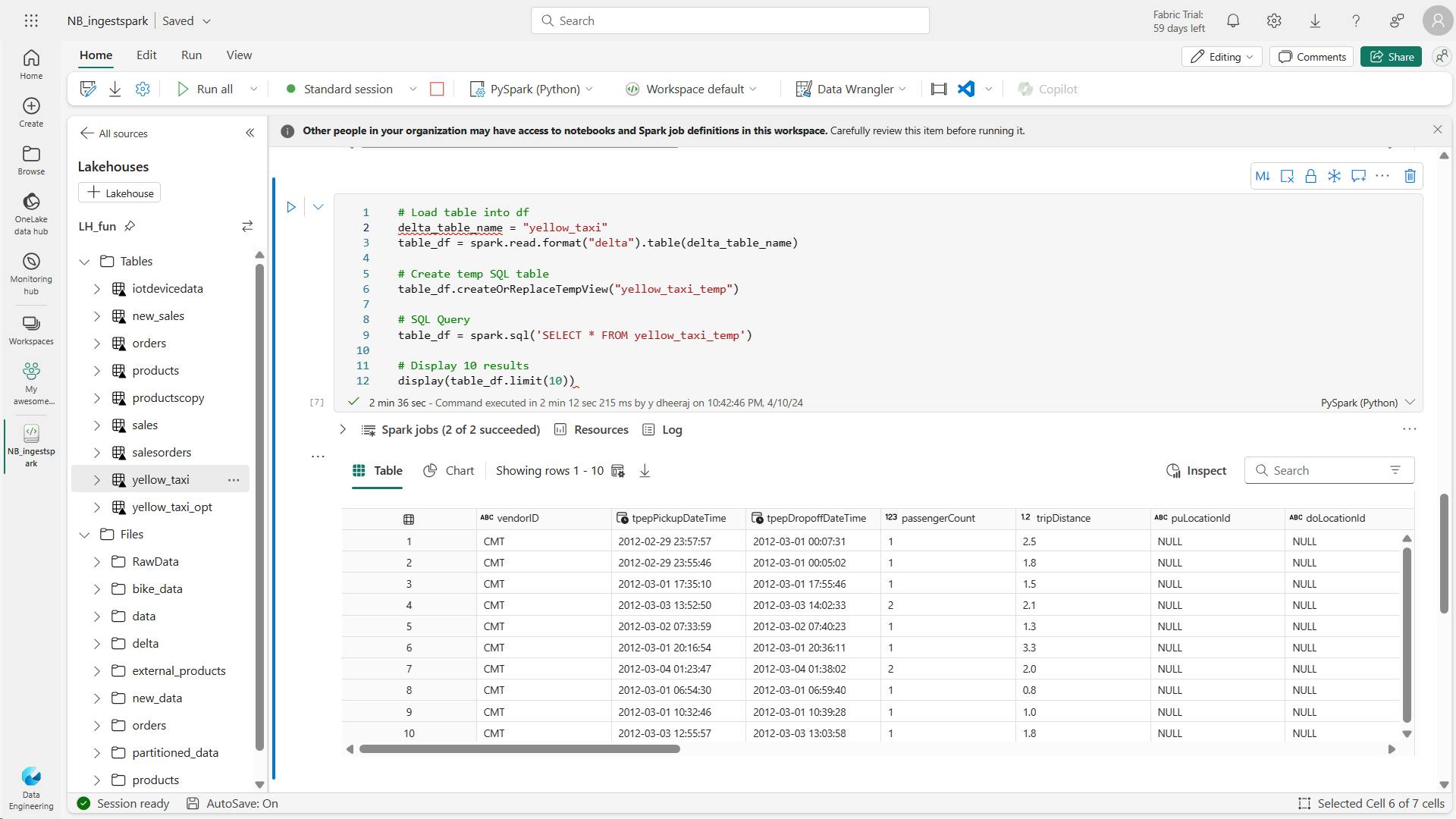
opt table:
 # Load table into df
 delta_table_name = "yellow_taxi_opt"
 opttable_df = spark.read.format("delta").table(delta_table_name)

 # Create temp SQL table
 opttable_df.createOrReplaceTempView("yellow_taxi_opt")

 # SQL Query to confirm
 opttable_df = spark.sql('SELECT * FROM yellow_taxi_opt')

 # Display results
 display(opttable_df.limit(10))
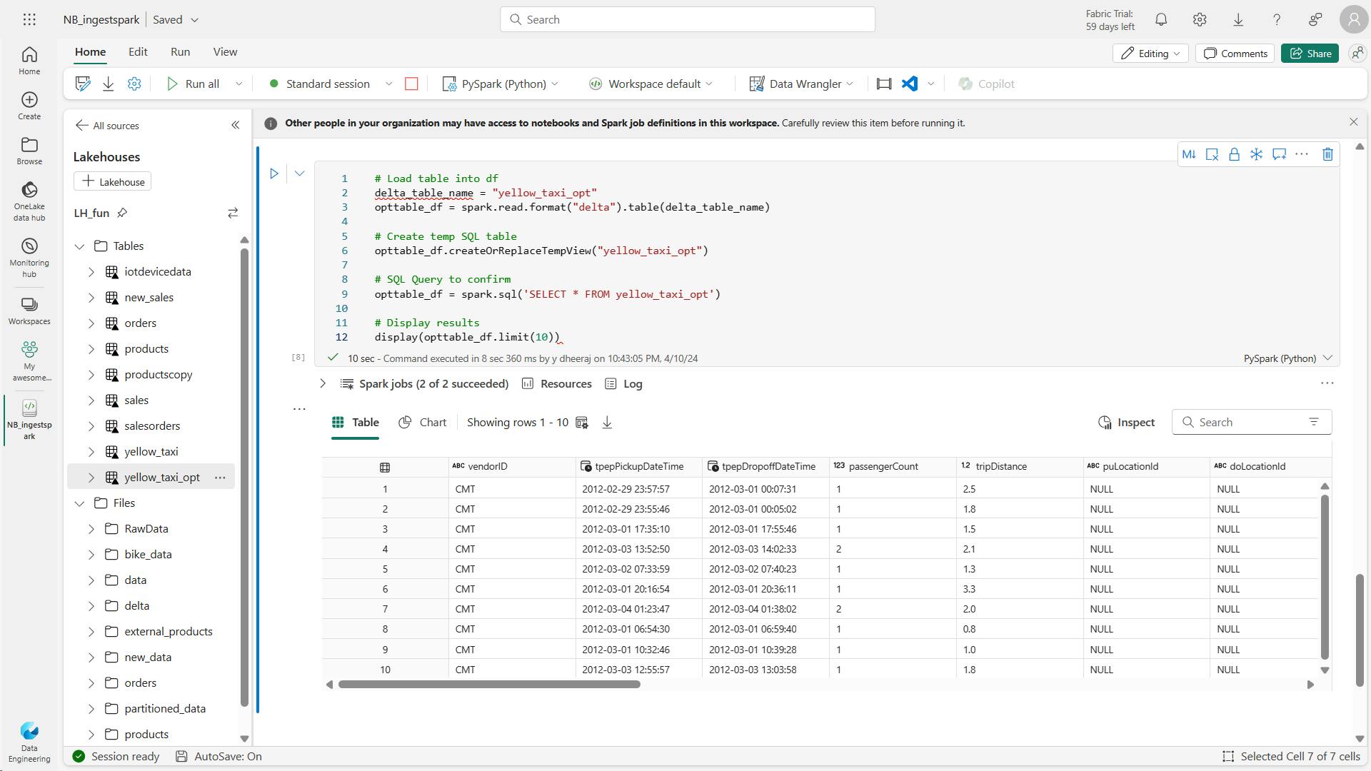
Notice the execution time difference between querying the table with non optimized data and a table with optimized data.
vii. Clean up resources
6. Knowledge check
What is the benefit of using Fabric notebooks over manual uploads for data ingestion?
Notebooks provide an automated approach to ingestion and transformation.
What is the purpose of V-Order and Optimize Write in Delta tables?
V-Order and Optimize Write enhance Delta tables by sorting data and creating fewer, larger Parquet files.
Why consider basic data cleansing when loading data into Fabric lakehouse?
Basic cleaning is done to ensure data quality and consistency before moving on to transformation and modeling steps.
7. Summary
In this module, you learned how to use Spark and Fabric notebooks to ingest data into a lakehouse.
Fabric notebooks offer automation and a comprehensive solution for ingestion and transformation. Fabric notebooks use a Spark engine to allow a multi-threaded, distributed transaction for speedy processes. Lakehouses support structured, semi-structured, and unstructured files and Delta tables. Optimize Delta table configuration for more performant reads and writes.
Before moving to the transformation and modeling steps, consider where to transform and how users interact with the data.
Learning objectives
By the end of this module, you’ll be able to:
Ingest external data to Fabric lakehouses using Spark
Configure external source authentication and optimization
Load data into lakehouse as files or as Delta tables
Optimize Delta table writes: V-Order, Optimize write
VIII. Organize a Fabric lakehouse using medallion architecture design
Explore the potential of the medallion architecture design in Microsoft Fabric. Organize and transform your data across Bronze, Silver, and Gold layers of a lakehouse for optimized analytics.
1. Introduction
The Fabric lakehouse, blending data lakes and data warehouses, offers an ideal platform to manage and analyze this data.
The medallion architecture has become a standard across the industry for lakehouse-based analytics.
In this module, you'll explore and build a medallion architecture for Fabric lakehouses, query and report on data in your Fabric lakehouse, and describe best practices for security and governance of your Fabric lakehouse.
2. Describe medallion architecture
Data lakehouses in Fabric are built on the Delta Lake format, which natively supports ACID (Atomicity, Consistency, Isolation, Durability) transactions.
Within this framework, the medallion architecture is a recommended data design pattern used to organize data in a lakehouse logically.
It aims to improve data quality as it moves through different layers. The architecture typically has three layers – bronze (raw), silver (validated), and gold (enriched), each representing higher data quality levels.
Some people also call it a "multi-hop" architecture, meaning that data can move between layers as needed.
i. Understand the medallion architecture format
a. Bronze layer
The bronze or raw layer of the medallion architecture is the first layer of the lakehouse.
It's the landing zone for all data, whether it's structured, semi-structured, or unstructured.
The data is stored in its original format, and no changes are made to it.
b. Silver layer
The silver or validated layer is the second layer of the lakehouse. It's where you'll validate and refine your data.
Typical activities in the silver layer include combining and merging data and enforcing data validation rules like removing nulls and deduplicating.
The silver layer can be thought of as a central repository across an organization or team, where data is stored in a consistent format and can be accessed by multiple teams.
In the silver layer you're cleaning your data enough so that everything is in one place and ready to be refined and modeled in the gold layer.
c. Gold layer
The gold or enriched layer is the third layer of the lakehouse.
In the gold layer, data undergoes further refinement to align with specific business and analytics needs. This could involve aggregating data to a particular granularity, such as daily or hourly, or enriching it with external information.
Once the data reaches the gold stage, it becomes ready for use by downstream teams, including analytics, data science, or MLOps.
ii. Customize your medallion architecture
Depending on your organization's specific use case, you may have a need for more layers.
For example, you might have an additional "raw" layer for landing data in a specific format before it's transformed into the bronze layer. Or you might have a "platinum" layer for data that's been further refined and enriched for a specific use case.
Regardless of the names and number of layers, the medallion architecture is flexible and can be tailored to meet your organization's particular requirements.
iii. Move data across layers in Fabric
Moving data across medallion layers refines, organizes, and prepares it for downstream data activities.
Within Fabric's lakehouse, there's more than one way to move data between layers, ensuring that you can choose the method that works for your team.
There are a few things to consider when deciding how to move and transform data across layers.
How much data are you working with?
How complex are the transformations you need to make?
How often will you need to move data between layers?
What tools are you most comfortable with?
Understanding the difference between data transformation and data orchestration helps you select the right tools for the job within Fabric.
a. Data transformation
Data transformation involves altering the structure or content of data to meet specific requirements.
Tools for data transformation in Fabric include Dataflows (Gen2) and notebooks.
1. Dataflows (Gen2)
Dataflows are a great option for smaller semantic models and simple transformations. Notebooks are a better option for larger semantic models and more complex transformations.
2. Notebooks
Notebooks also allow you to save your transformed data as a managed Delta table in the lakehouse, ready for reporting.
b. Data orchestration
Data orchestration refers to the coordination and management of multiple data-related processes, ensuring they work together to achieve a desired outcome.
The primary tool for data orchestration in Fabric is pipelines.
i. Pipeline
A pipeline is a series of steps that move data from one place to another, in this case, from one layer of the medallion architecture to the next.
Pipelines can be automated to run on a schedule or triggered by an event.
3. Implement a medallion architecture in Fabric
Now that you have a solid understanding of the medallion architecture, let's explore how to put it into action within Fabric.
i. Set up the foundation:
Create your Fabric lakehouse. You can use the same lakehouse for multiple medallion architectures, or alternatively, you can use different lakehouses and even different lakehouses in different workspaces, depending on your use case. We'll dive more into this in unit 5.
ii. Design your architecture
Create your architecture layout, define your layers, and determine how data will flow between them.
The most straightforward implementation is to use Bronze as the raw layer, Silver as the curated layer, and gold as the presentation layer.
Your gold layer should be modeled in a star schema and optimized for reporting.
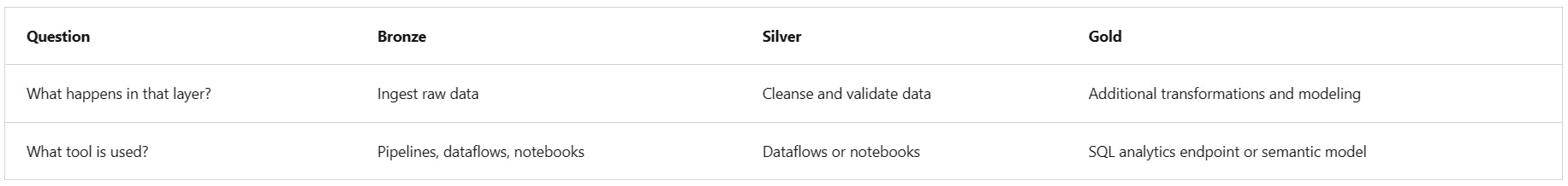
iii. Ingest data into bronze
Determine how you'll ingest data into your bronze layer.
You can do this using pipelines, dataflows, or notebooks.
iv. Transform data and load to silver
Determine how you'll transform data in your silver layer. You can do this using dataflows or notebooks.
Transformations at the silver level should be focused on data quality and consistency, not on data modeling.
v. Generate a gold layer
Determine how you'll generate your gold layer(s), what it will contain, and how it will be used.
The gold layer is where you'll model your data for reporting using a dimensional model. Here you'll establish relationships, define measures, and incorporate any other elements essential for effective reporting.
You can have multiple gold layers for different audiences or domains. For example, you might have a gold layer for your finance team and a separate gold layer for your sales team. You might also have a gold layer for your data scientists that is optimized for machine learning.
Depending on your needs, you might also use a Data Warehouse as your gold layer. See Get started with data warehouses in Microsoft Fabric to learn more.
In Fabric, you can transform your data using dataflows or notebooks, and then load it into a gold Delta table in the lakehouse. You can then connect to the Delta table using a SQL analytics endpoint and use SQL to model your data for reporting. Alternatively, you can use Power BI to connect to the SQL analytics endpoint of the gold layer and model your data for reporting.
vi. Enable downstream consumption
Determine how you'll enable downstream consumption of your data. You can do this using workspace or item permissions, or by connecting to the SQL analytics endpoint.
4. Query and report on data in your Fabric lakehouse
Now that your medallion architecture is in place, data teams and the business can start using it to query and report on data.
Fabric has several tools and technologies that enable you to query and report on data in your lakehouse, including SQL analytics endpoints and Direct Lake mode in Power BI semantic models.
i. Query data in your lakehouse
Teams can use SQL to explore and query data in the gold layer.
You can analyze data in delta tables at any layer of the medallion architecture using the T-SQL language, save functions, generate views, and apply SQL security.
You can also use the SQL analytics endpoint to connect to your lakehouse from third-party tools and applications.
The SQL analytics endpoint in Fabric enables you to write queries, manage the semantic model, and query data using the new visual query experience.
Note:
The SQL analytics endpoint operates in read-only mode over lakehouse delta tables. To modify data in your lakehouse you can use dataflows, notebooks, or pipelines.
In addition to using the SQL analytics endpoint for data exploration, you can also create a Power BI semantic model in Direct Lake mode to query data in your lakehouse.
When you create a lakehouse, the system also provisions an associated default semantic model. The default semantic model is a semantic model with metrics on top of lakehouse data.
Direct Lake mode
When a Power BI report displays a data element, it fetches it from the underlying semantic model, which in turn accesses a lakehouse for data retrieval.
To enhance efficiency, the default semantic model preloads frequently requested data into the cache and updates it as necessary.
This approach is called Direct Lake mode and truly gives you the best of both worlds: the performance of a semantic model and the freshness of lakehouse data.
ii. Tailor your medallion layers for different needs
Tailoring medallion layers to different needs allows you to optimize data processing and access for specific use cases. By customizing these layers, you can ensure that each layer's structure and organization align with the requirements of different user groups, improving performance, ease of use, and data relevance for diverse stakeholders.
Creating multiple Gold layers tailored for diverse audiences or domains highlights the flexibility of the medallion architecture. Finance, sales, data science – each can have its optimized Gold layer, serving specific analytical requirements.
Some applications, third-party tools, or systems require specific data formats. You can utilize your medallion architecture to generate cleansed and properly formatted data.
5. Considerations for managing your lakehouse
There are a couple of considerations to keep in mind when managing your lakehouse, including
how to secure your lakehouse and
how to handle continuous integration and continuous delivery (CI/CD).
i. Secure your lakehouse
Secure your lakehouse by ensuring that only authorized users can access data.
In Fabric, you can do this by setting permissions at the workspace or item level.
ii. Considerations for Continuous Integration and Continuous Delivery (CI/CD)
Designing a Continuous Integration/Continuous Deployment (CI/CD) process for a lakehouse architecture involves several considerations to ensure a smooth and efficient deployment process.
Considerations include implementing data quality checks, version control, automated deployments, monitoring, and security measures.
Considerations should also include scalability, disaster recovery, collaboration, compliance, and continuous improvement to ensure reliable and efficient data pipeline deployments.
While some of these are related to processes and practices, others are related to the tools and technologies used to implement CI/CD.
Fabric natively provides several tools and technologies to support CI/CD processes.
6. Exercise - Organize your Fabric lakehouse using a medallion architecture
create a lakehouse in Fabric and move data through the medallion architecture.
You'll also learn how to query and report on data in your Fabric lakehouse.
In this exercise you will build out a medallion architecture in a Fabric lakehouse using notebooks. You will create a workspace, create a lakehouse, upload data to the bronze layer, transform the data and load it to the silver Delta table, transform the data further and load it to the gold Delta tables, and then explore the semantic model and create relationships.
i. Create a workspace
Navigate to the workspace settings and enable the Data model editing preview feature.
This will enable you to create relationships between tables in your lakehouse using a Power BI semantic model.
ii. Create a lakehouse and upload data to bronze layer
Data: orders zip [Link]
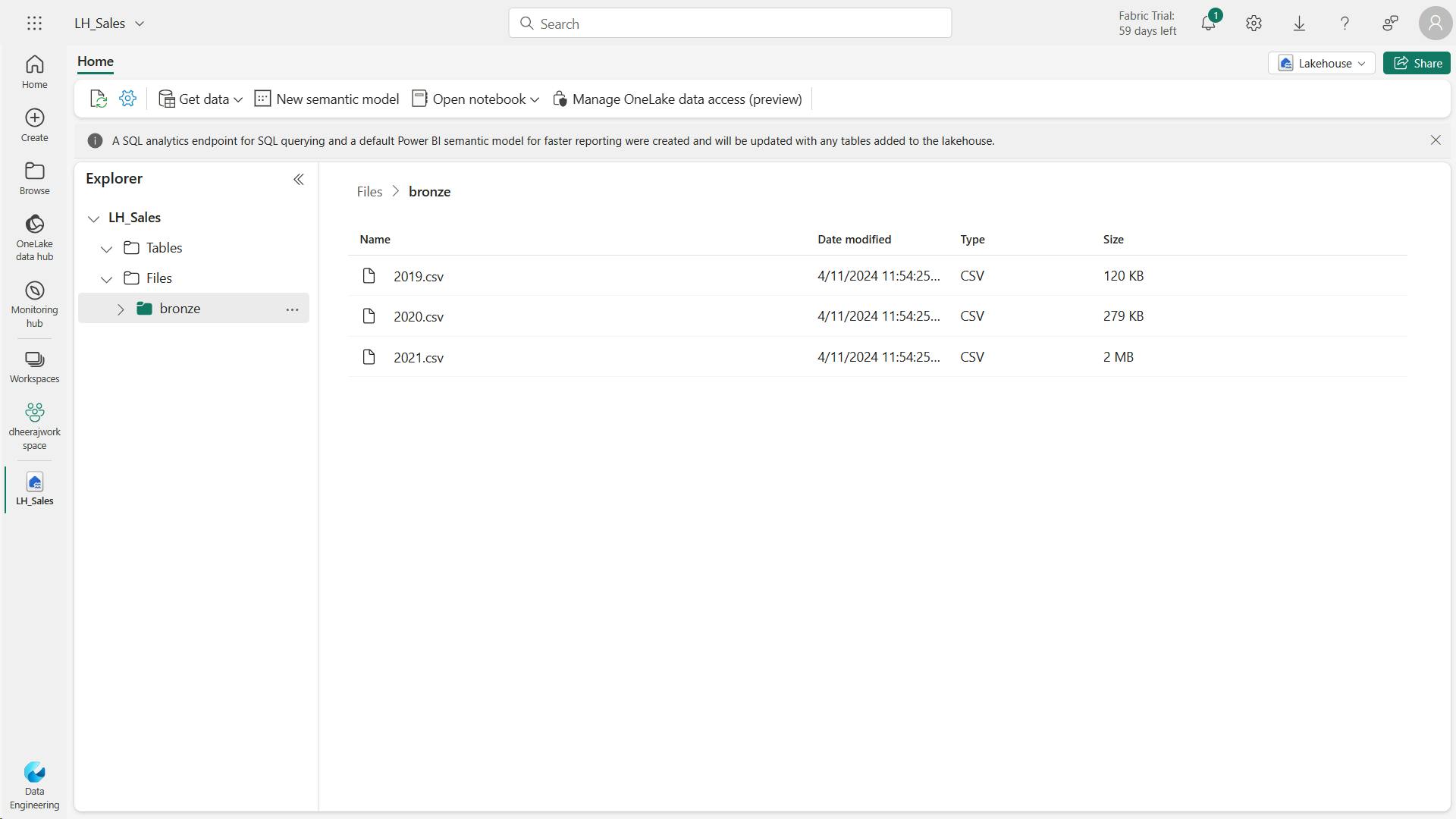
iii. Transform data and load to silver Delta table
use a notebook to transform the data and load it to a delta table in the silver layer.
 from pyspark.sql.types import *

 # Create the schema for the table
 orderSchema = StructType([
     StructField("SalesOrderNumber", StringType()),
     StructField("SalesOrderLineNumber", IntegerType()),
     StructField("OrderDate", DateType()),
     StructField("CustomerName", StringType()),
     StructField("Email", StringType()),
     StructField("Item", StringType()),
     StructField("Quantity", IntegerType()),
     StructField("UnitPrice", FloatType()),
     StructField("Tax", FloatType())
     ])

 # Import all files from bronze folder of lakehouse
 df = spark.read.format("csv").option("header", "true").schema(orderSchema).load("Files/bronze/*.csv")

 # Display the first 10 rows of the dataframe to preview your data
 display(df.head(10))
The code ran loaded the data from the CSV files in the bronze folder into a Spark dataframe, and then displayed the first few rows of the dataframe.
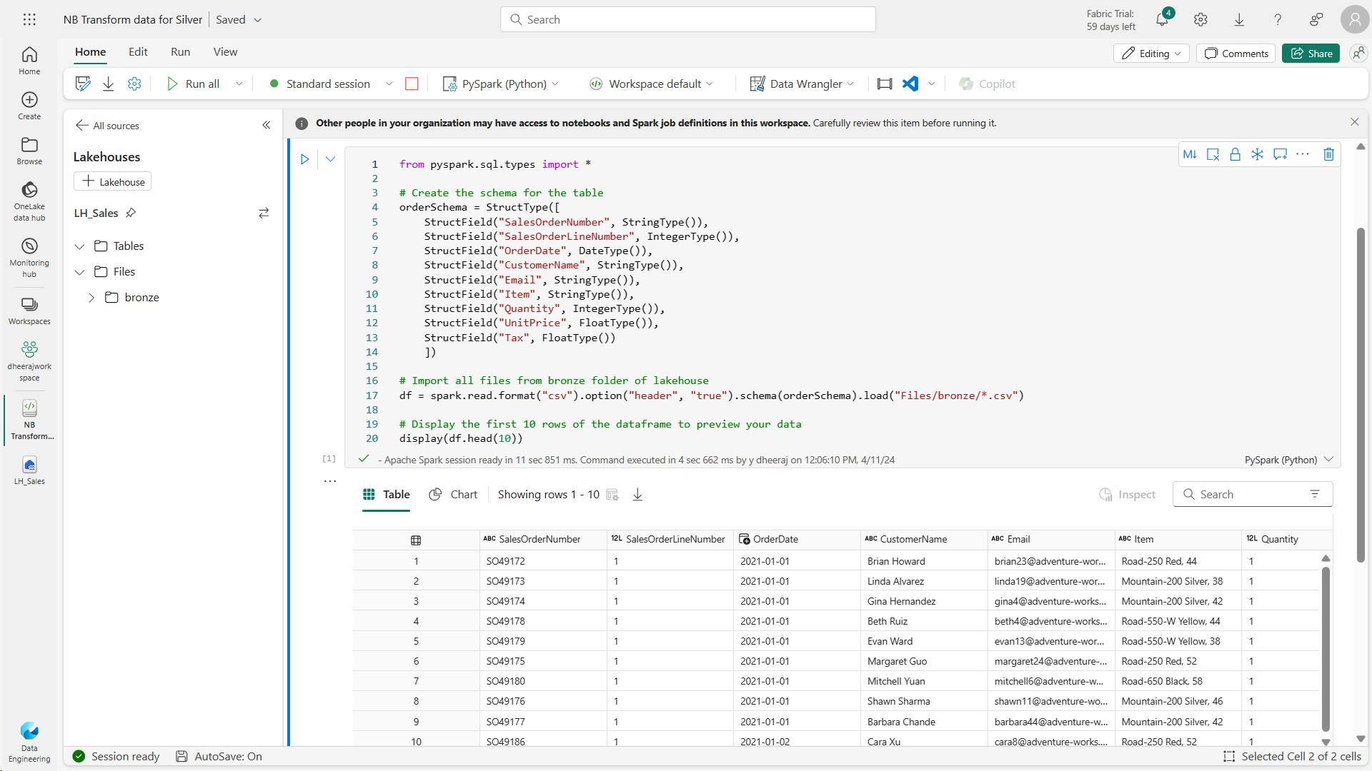
Now you’ll add columns for data validation and cleanup, using a PySpark dataframe to add columns and update the values of some of the existing columns.
 from pyspark.sql.functions import when, lit, col, current_timestamp, input_file_name

 # Add columns IsFlagged, CreatedTS and ModifiedTS
 df = df.withColumn("FileName", input_file_name()) \
     .withColumn("IsFlagged", when(col("OrderDate") < '2019-08-01',True).otherwise(False)) \
     .withColumn("CreatedTS", current_timestamp()).withColumn("ModifiedTS", current_timestamp())

 # Update CustomerName to "Unknown" if CustomerName null or empty
 df = df.withColumn("CustomerName", when((col("CustomerName").isNull() | (col("CustomerName")=="")),lit("Unknown")).otherwise(col("CustomerName")))
Finally, you’re updating the CustomerName column to “Unknown” if it’s null or empty.
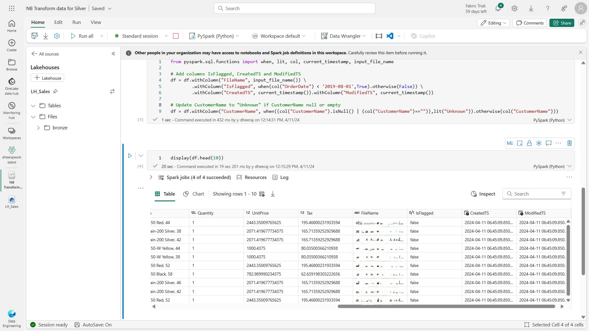
Define the schema for the sales_silver table in the sales database using Delta Lake format.
 # Define the schema for the sales_silver table

 from pyspark.sql.types import *
 from delta.tables import *

 DeltaTable.createIfNotExists(spark) \
     .tableName("sales.sales_silver") \
     .addColumn("SalesOrderNumber", StringType()) \
     .addColumn("SalesOrderLineNumber", IntegerType()) \
     .addColumn("OrderDate", DateType()) \
     .addColumn("CustomerName", StringType()) \
     .addColumn("Email", StringType()) \
     .addColumn("Item", StringType()) \
     .addColumn("Quantity", IntegerType()) \
     .addColumn("UnitPrice", FloatType()) \
     .addColumn("Tax", FloatType()) \
     .addColumn("FileName", StringType()) \
     .addColumn("IsFlagged", BooleanType()) \
     .addColumn("CreatedTS", DateType()) \
     .addColumn("ModifiedTS", DateType()) \
     .execute()
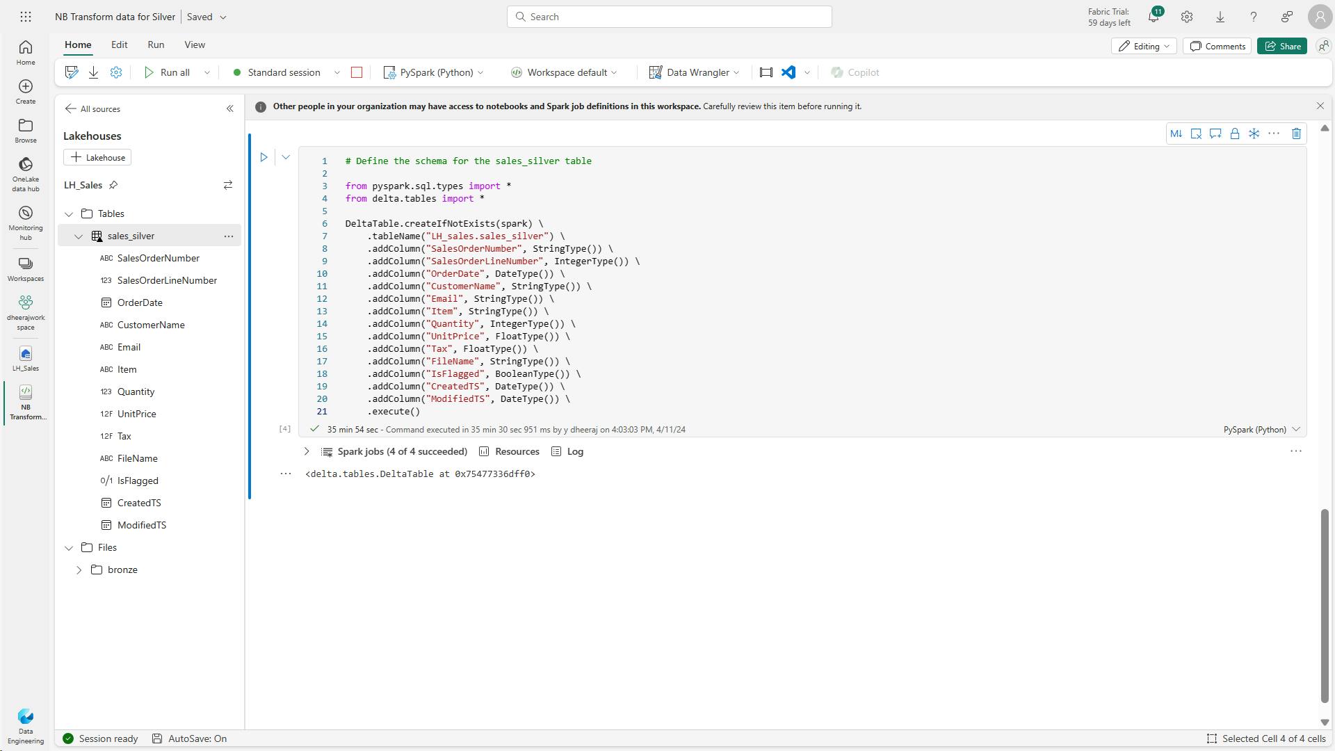
Upsert operation on a Delta table, updating existing records based on specific conditions and inserting new records when no match is found.
Now you’re going to perform an upsert operation on a Delta table, updating existing records based on specific conditions and inserting new records when no match is found.
# Update existing records and insert new ones based on a condition defined by the columns SalesOrderNumber, OrderDate, CustomerName, and Item.

from delta.tables import *

deltaTable = DeltaTable.forPath(spark, 'Tables/sales_silver')

dfUpdates = df

deltaTable.alias('silver') \
  .merge(
    dfUpdates.alias('updates'),
    'silver.SalesOrderNumber = updates.SalesOrderNumber and silver.OrderDate = updates.OrderDate and silver.CustomerName = updates.CustomerName and silver.Item = updates.Item'
  ) \
   .whenMatchedUpdate(set =
    {

    }
  ) \
 .whenNotMatchedInsert(values =
    {
      "SalesOrderNumber": "updates.SalesOrderNumber",
      "SalesOrderLineNumber": "updates.SalesOrderLineNumber",
      "OrderDate": "updates.OrderDate",
      "CustomerName": "updates.CustomerName",
      "Email": "updates.Email",
      "Item": "updates.Item",
      "Quantity": "updates.Quantity",
      "UnitPrice": "updates.UnitPrice",
      "Tax": "updates.Tax",
      "FileName": "updates.FileName",
      "IsFlagged": "updates.IsFlagged",
      "CreatedTS": "updates.CreatedTS",
      "ModifiedTS": "updates.ModifiedTS"
    }
  ) \
  .execute()
This operation is important because it enables you to update existing records in the table based on the values of specific columns, and insert new records when no match is found.
This is a common requirement when you’re loading data from a source system that may contain updates to existing and new records.
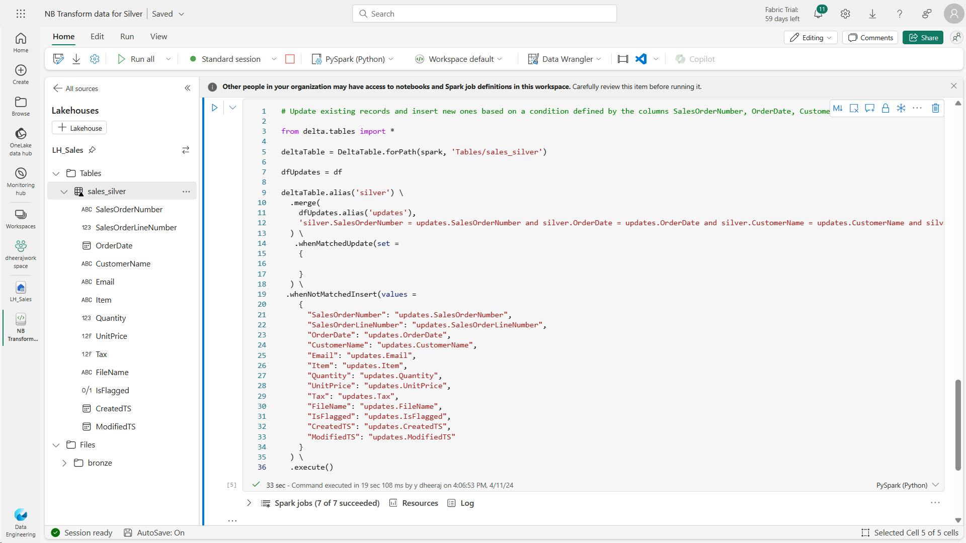
iv. Explore data in the silver layer using the SQL endpoint
Now that you have data in your silver layer, you can use the SQL endpoint to explore the data and perform some basic analysis.
This is a nice option for you if you’re familiar with SQL and want to do some basic exploration of your data. In this exercise we’re using the SQL endpoint view in Fabric, but note that you can also use other tools like SQL Server Management Studio (SSMS) and Azure Data Explorer.
SELECT
    YEAR(OrderDate) AS Year,
    CAST (SUM(Quantity * (UnitPrice + Tax)) AS DECIMAL(12, 2)) AS TotalSales
FROM sales_silver
GROUP BY YEAR(OrderDate)
ORDER BY YEAR(OrderDate)
This query calculates the total sales for each year in the sales_silver table.
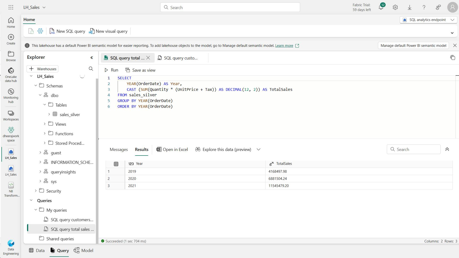
Now we’ll take a look at which customers are purchasing the most (in terms of quantity)
 SELECT TOP 10 CustomerName, SUM(Quantity) AS TotalQuantity
 FROM sales_silver
 GROUP BY CustomerName
 ORDER BY TotalQuantity DESC
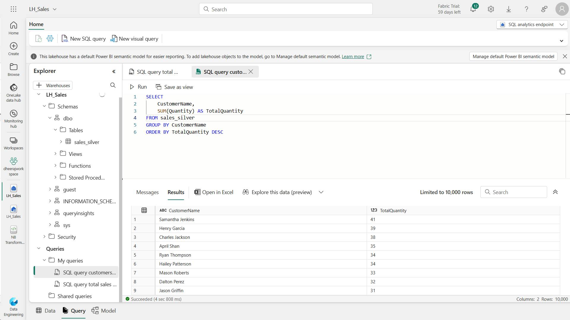
Data exploration at the silver layer is useful for basic analysis, but you’ll need to transform the data further and model it into a star schema to enable more advanced analysis and reporting. You’ll do that in the next section.
v. Transform data for gold layer
You have successfully taken data from your bronze layer, transformed it, and loaded it into a silver Delta table.
Now you’ll use a new notebook to transform the data further, model it into a star schema, and load it into gold Delta tables.
Note that you could have done all of this in a single notebook, but for the purposes of this exercise you’re using separate notebooks to demonstrate the process of transforming data from bronze to silver and then from silver to gold.
This can help with debugging, troubleshooting, and reuse.
a. Code to load data to your dataframe and start building out your star schema:
 # Load data to the dataframe as a starting point to create the gold layer
 df = spark.read.table("sales_silver")
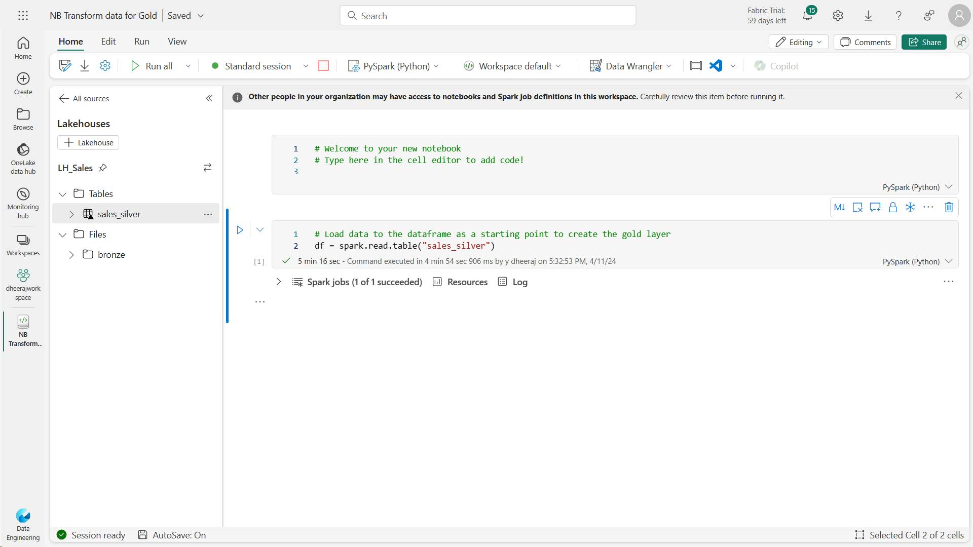
Date dimension table:
b. code to create your date dimension table:
 from pyspark.sql.types import *
 from delta.tables import *

 # Define the schema for the dimdate_gold table
 DeltaTable.createIfNotExists(spark) \
     .tableName("dimdate_gold") \
     .addColumn("OrderDate", DateType()) \
     .addColumn("Day", IntegerType()) \
     .addColumn("Month", IntegerType()) \
     .addColumn("Year", IntegerType()) \
     .addColumn("mmmyyyy", StringType()) \
     .addColumn("yyyymm", StringType()) \
     .execute()
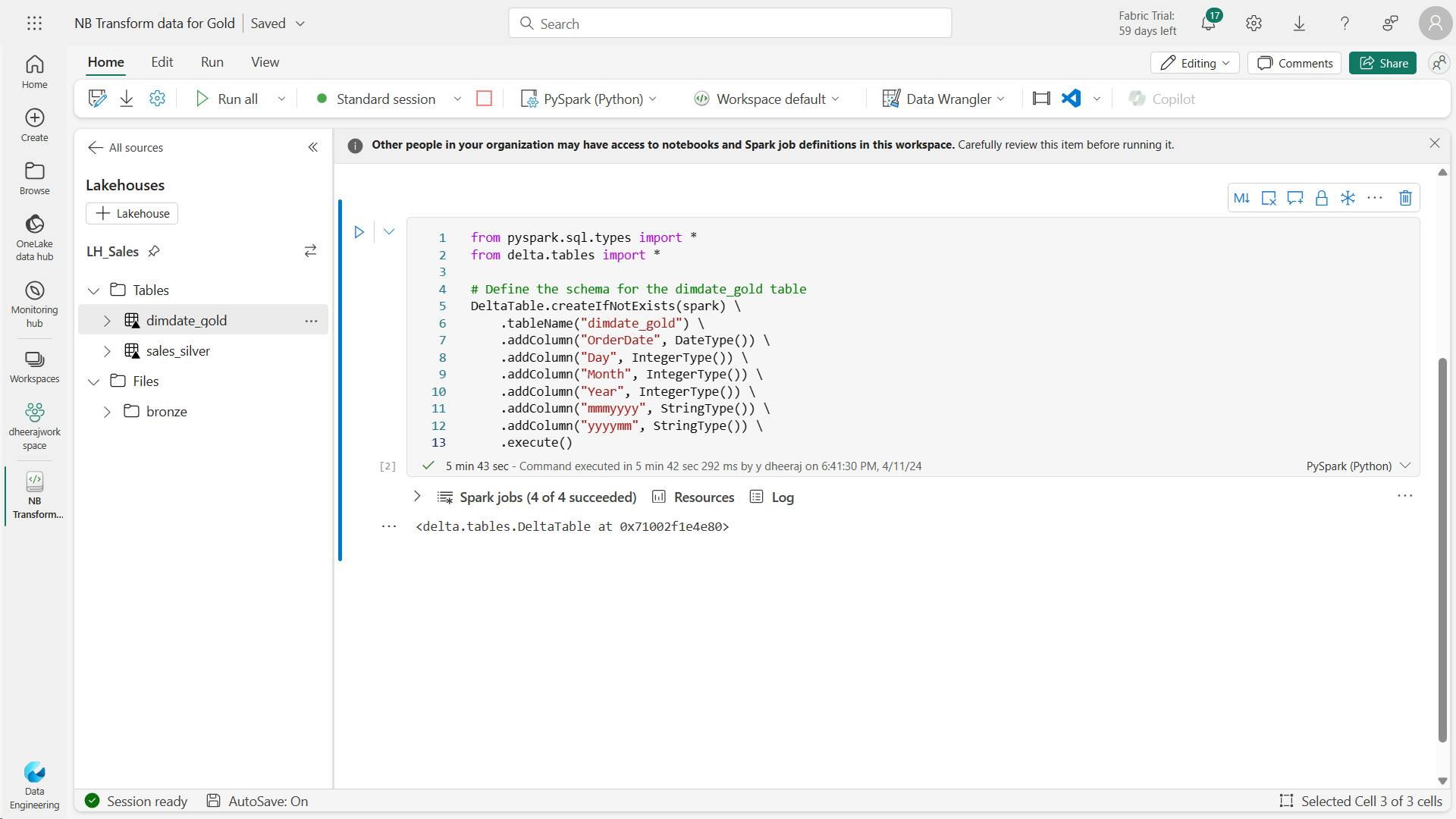
c. Code to create a dataframe for your date dimension, dimdate_gold
 from pyspark.sql.functions import col, dayofmonth, month, year, date_format

 # Create dataframe for dimDate_gold

 dfdimDate_gold = df.dropDuplicates(["OrderDate"]).select(col("OrderDate"), \
         dayofmonth("OrderDate").alias("Day"), \
         month("OrderDate").alias("Month"), \
         year("OrderDate").alias("Year"), \
         date_format(col("OrderDate"), "MMM-yyyy").alias("mmmyyyy"), \
         date_format(col("OrderDate"), "yyyyMM").alias("yyyymm"), \
     ).orderBy("OrderDate")

 # Display the first 10 rows of the dataframe to preview your data

 display(dfdimDate_gold.head(10))
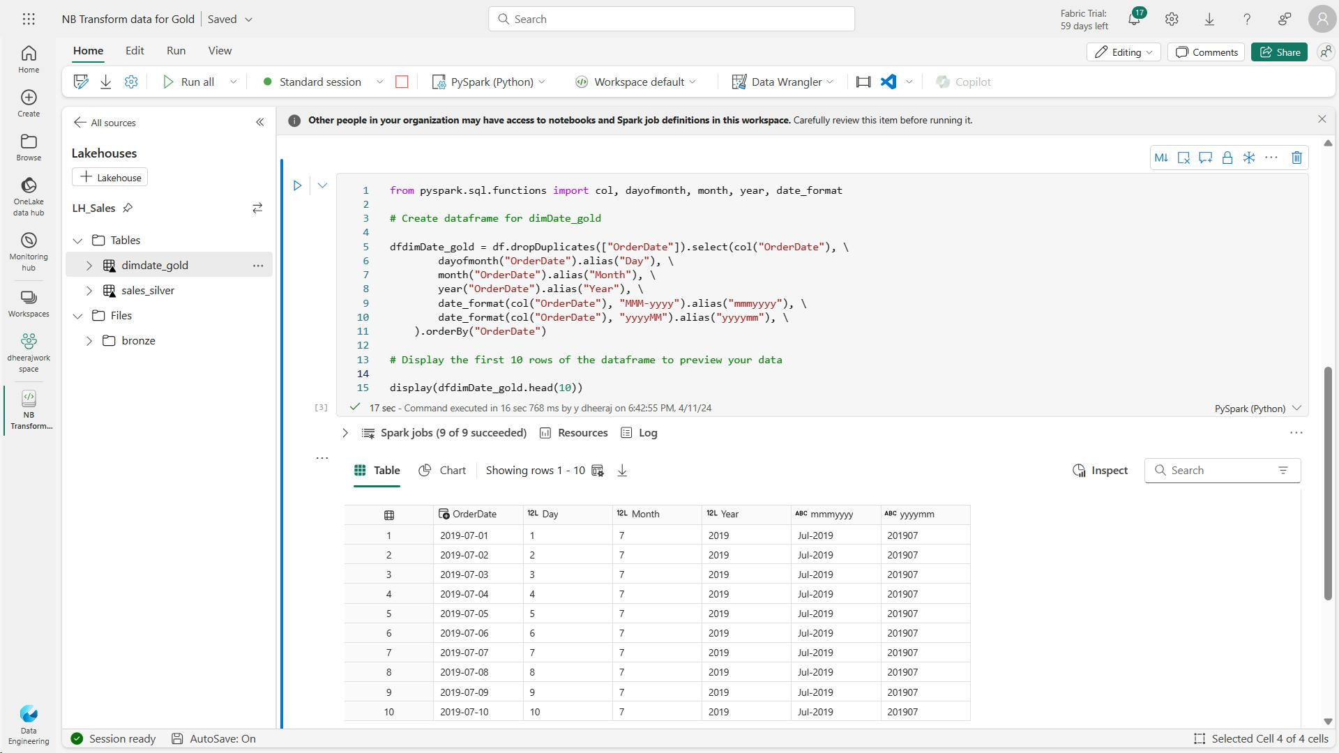
d. Code to update the date dimension as new data comes in:
 from delta.tables import *

 deltaTable = DeltaTable.forPath(spark, 'Tables/dimdate_gold')

 dfUpdates = dfdimDate_gold

 deltaTable.alias('silver') \
   .merge(
     dfUpdates.alias('updates'),
     'silver.OrderDate = updates.OrderDate'
   ) \
    .whenMatchedUpdate(set =
     {

     }
   ) \
  .whenNotMatchedInsert(values =
     {
       "OrderDate": "updates.OrderDate",
       "Day": "updates.Day",
       "Month": "updates.Month",
       "Year": "updates.Year",
       "mmmyyyy": "updates.mmmyyyy",
       "yyyymm": "yyyymm"
     }
   ) \
   .execute()
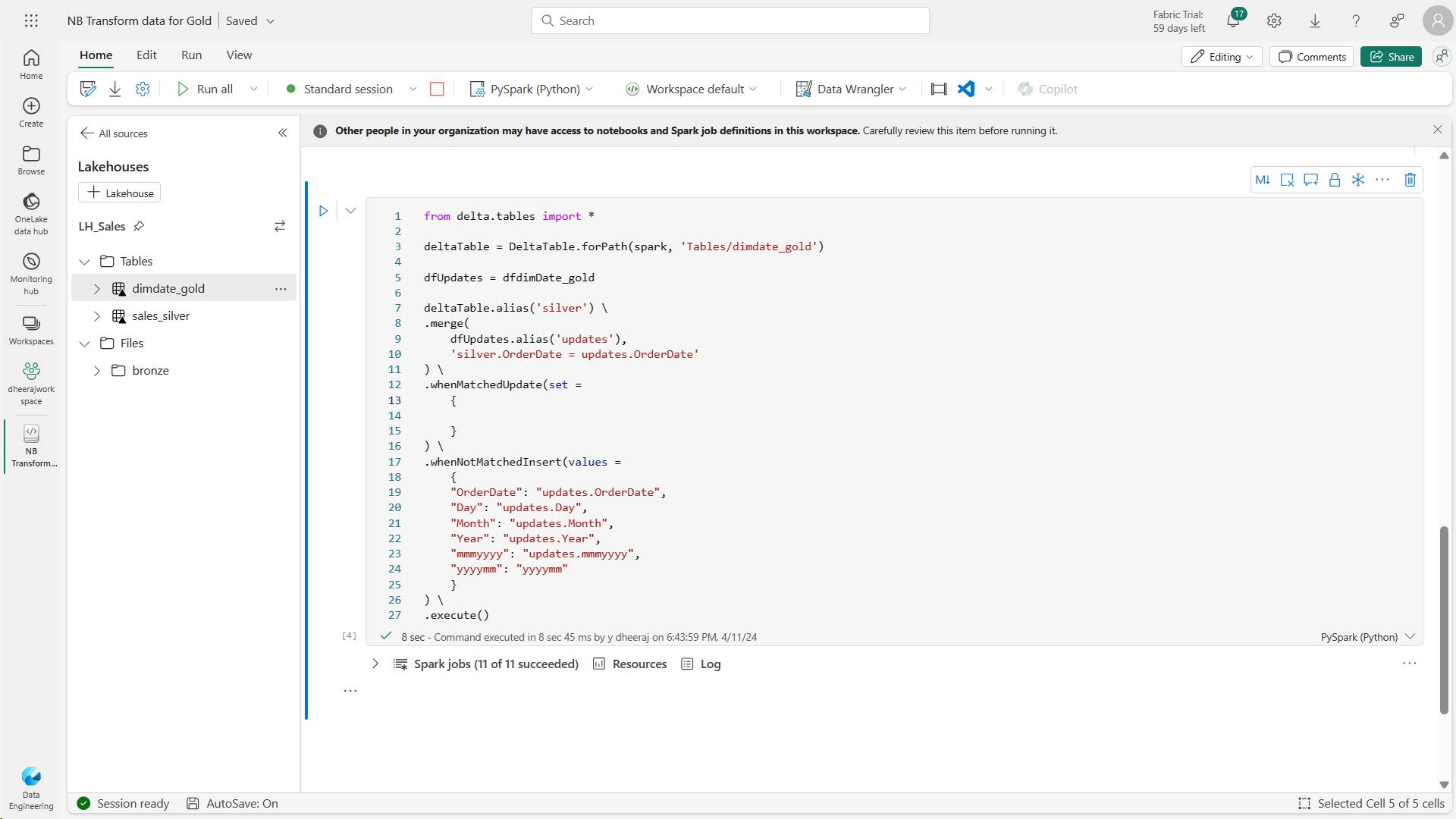
Customer dimension table:
e. Code to build out the customer dimension table
 from pyspark.sql.types import *
 from delta.tables import *

 # Create customer_gold dimension delta table
 DeltaTable.createIfNotExists(spark) \
     .tableName("dimcustomer_gold") \
     .addColumn("CustomerName", StringType()) \
     .addColumn("Email",  StringType()) \
     .addColumn("First", StringType()) \
     .addColumn("Last", StringType()) \
     .addColumn("CustomerID", LongType()) \
     .execute()
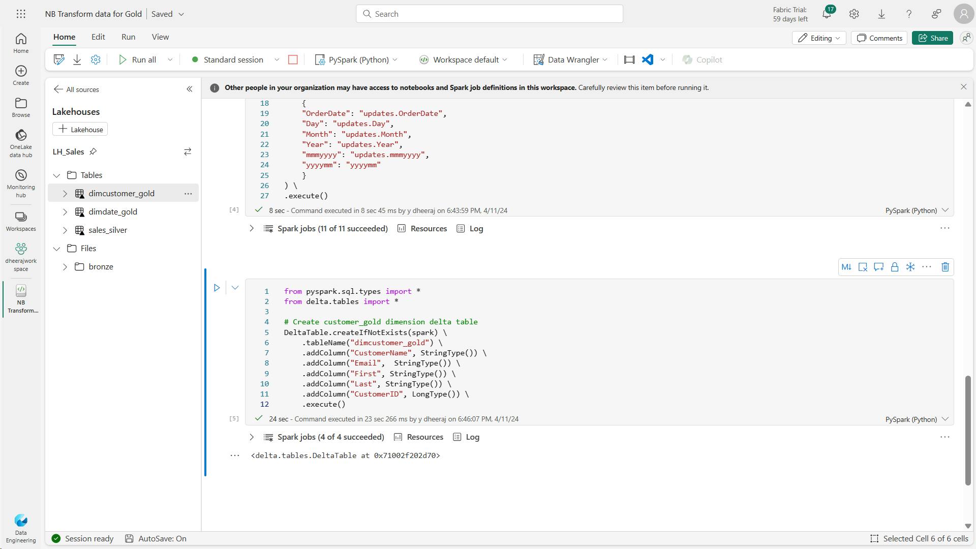
f. Code to drop duplicate customers, select specific columns, and split the “CustomerName” column to create “First” and “Last” name columns:
Here you have created a new DataFrame dfdimCustomer_silver by performing various transformations such as dropping duplicates, selecting specific columns, and splitting the “CustomerName” column to create “First” and “Last” name columns.
The result is a DataFrame with cleaned and structured customer data, including separate “First” and “Last” name columns extracted from the “CustomerName” column.
 from pyspark.sql.functions import col, split

 # Create customer_silver dataframe

 dfdimCustomer_silver = df.dropDuplicates(["CustomerName","Email"]).select(col("CustomerName"),col("Email")) \
     .withColumn("First",split(col("CustomerName"), " ").getItem(0)) \
     .withColumn("Last",split(col("CustomerName"), " ").getItem(1))

 # Display the first 10 rows of the dataframe to preview your data

 display(dfdimCustomer_silver.head(10))
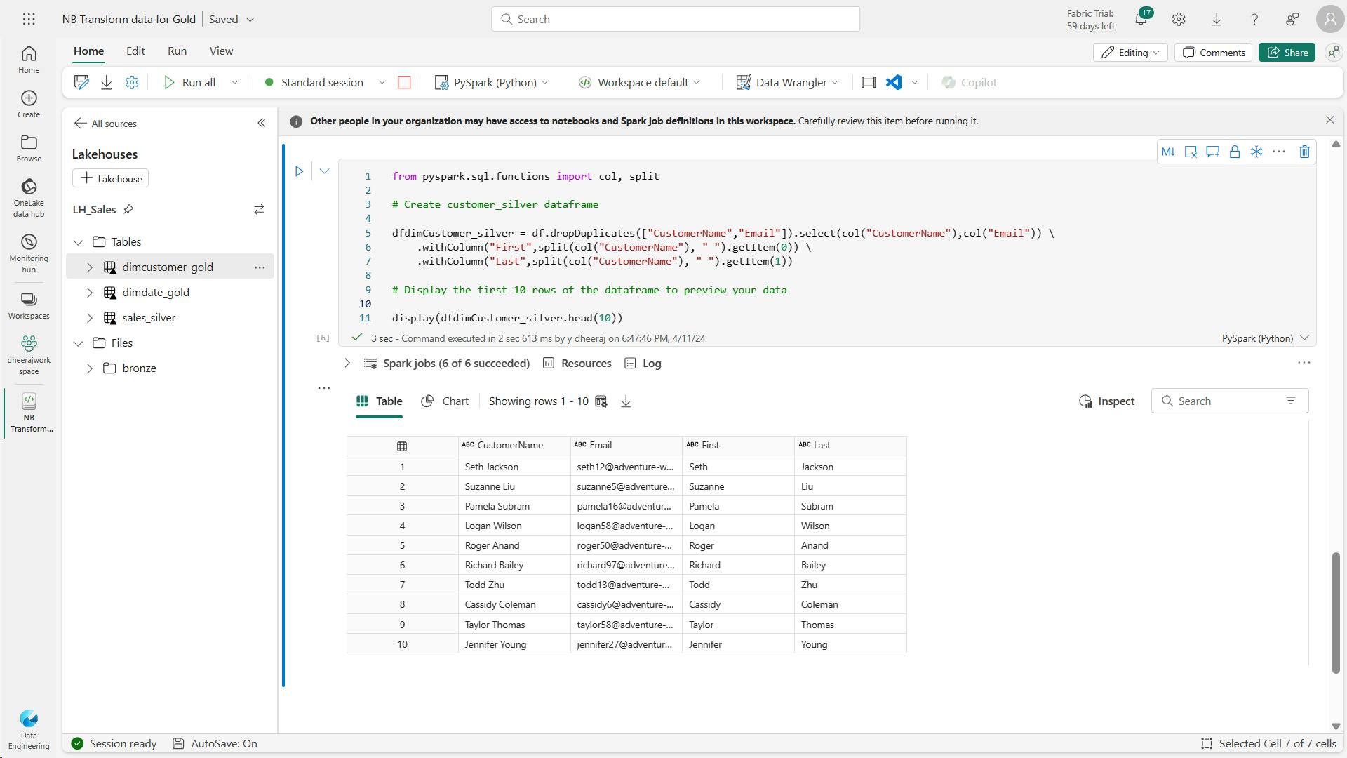
g. Code to create the ID column for our customers
Here you’re cleaning and transforming customer data (dfdimCustomer_silver) by performing a left anti join to exclude duplicates that already exist in the dimCustomer_gold table, and then generating unique CustomerID values using the monotonically_increasing_id() function.
 from pyspark.sql.functions import monotonically_increasing_id, col, when, coalesce, max, lit

 dfdimCustomer_temp = spark.read.table("dimcustomer_gold")

 MAXCustomerID = dfdimCustomer_temp.select(coalesce(max(col("CustomerID")),lit(0)).alias("MAXCustomerID")).first()[0]

 dfdimCustomer_gold = dfdimCustomer_silver.join(dfdimCustomer_temp,(dfdimCustomer_silver.CustomerName == dfdimCustomer_temp.CustomerName) & (dfdimCustomer_silver.Email == dfdimCustomer_temp.Email), "left_anti")

 dfdimCustomer_gold = dfdimCustomer_gold.withColumn("CustomerID",monotonically_increasing_id() + MAXCustomerID + 1)

 # Display the first 10 rows of the dataframe to preview your data

 display(dfdimCustomer_gold.head(10))
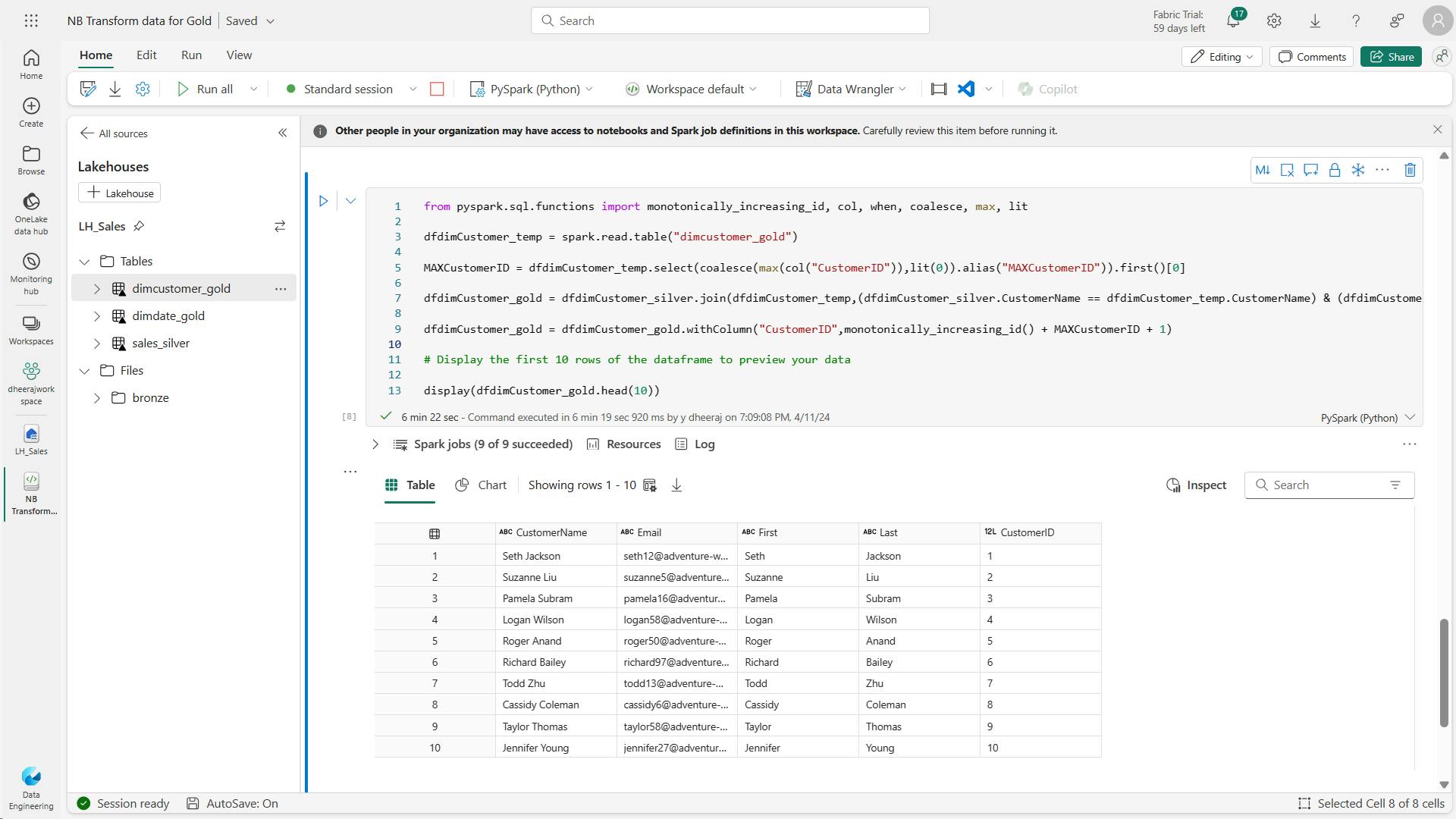
h. Code to ensure that your customer table remains up-to-date as new data comes in
from delta.tables import *

deltaTable = DeltaTable.forPath(spark, 'Tables/dimcustomer_gold')

dfUpdates = dfdimCustomer_gold

deltaTable.alias('silver') \
  .merge(
    dfUpdates.alias('updates'),
    'silver.CustomerName = updates.CustomerName AND silver.Email = updates.Email'
  ) \
   .whenMatchedUpdate(set =
    {

    }
  ) \
 .whenNotMatchedInsert(values =
    {
      "CustomerName": "updates.CustomerName",
      "Email": "updates.Email",
      "First": "updates.First",
      "Last": "updates.Last",
      "CustomerID": "updates.CustomerID"
    }
  ) \
  .execute()
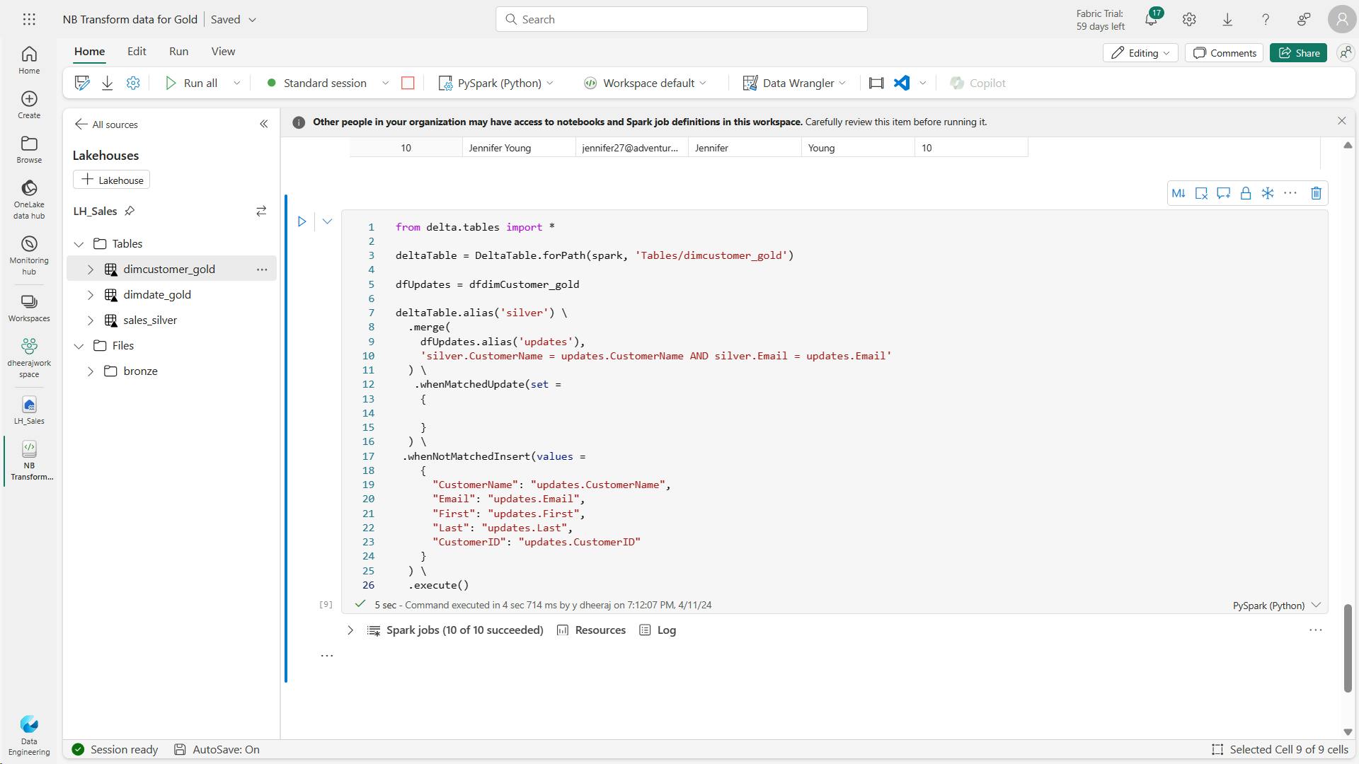
customer table
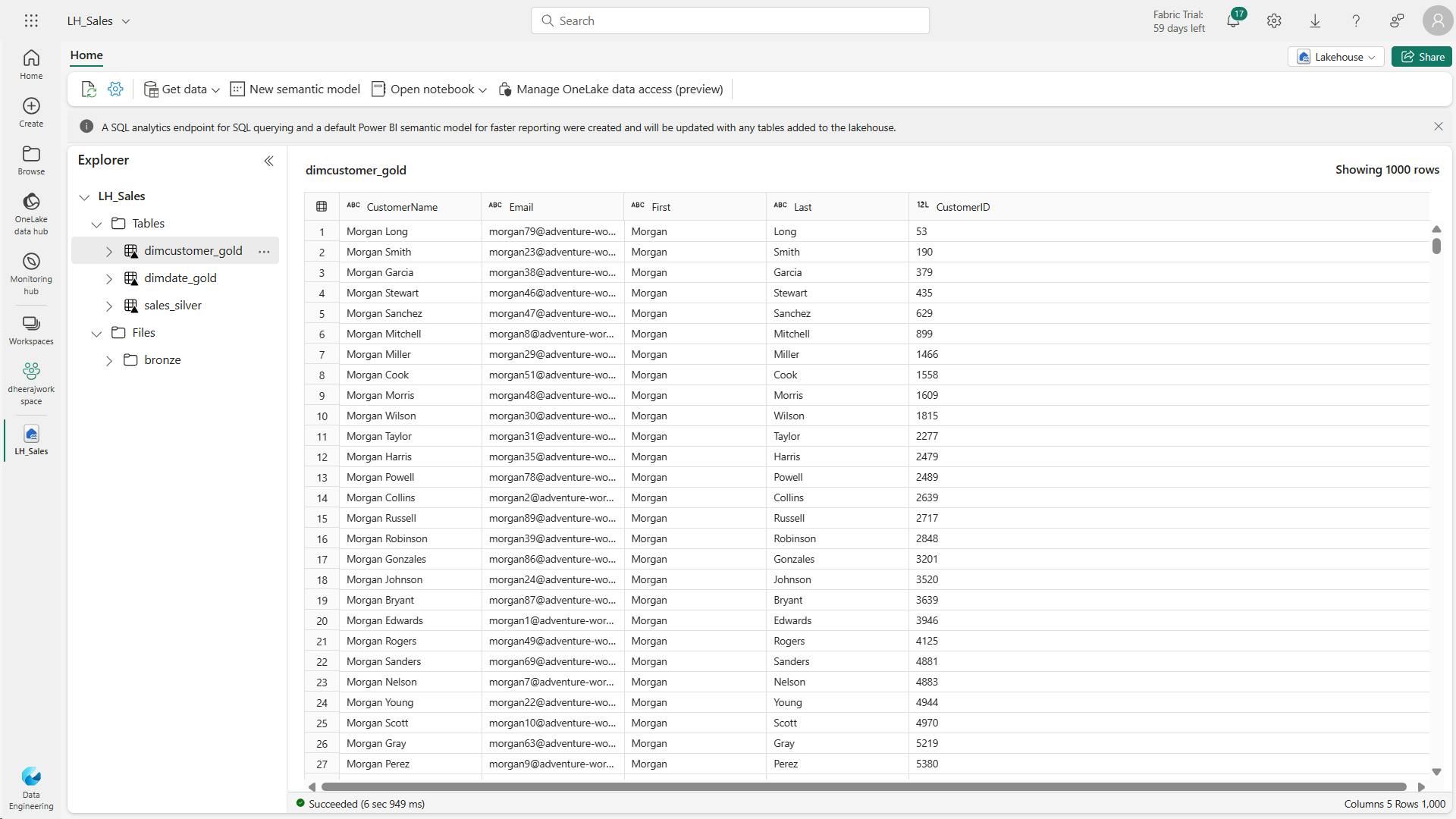
Product dimension table:
i. Code to create your product dimension
from pyspark.sql.types import *
from delta.tables import *

DeltaTable.createIfNotExists(spark) \
    .tableName("dimproduct_gold") \
    .addColumn("ItemName", StringType()) \
    .addColumn("ItemID", LongType()) \
    .addColumn("ItemInfo", StringType()) \
    .execute()
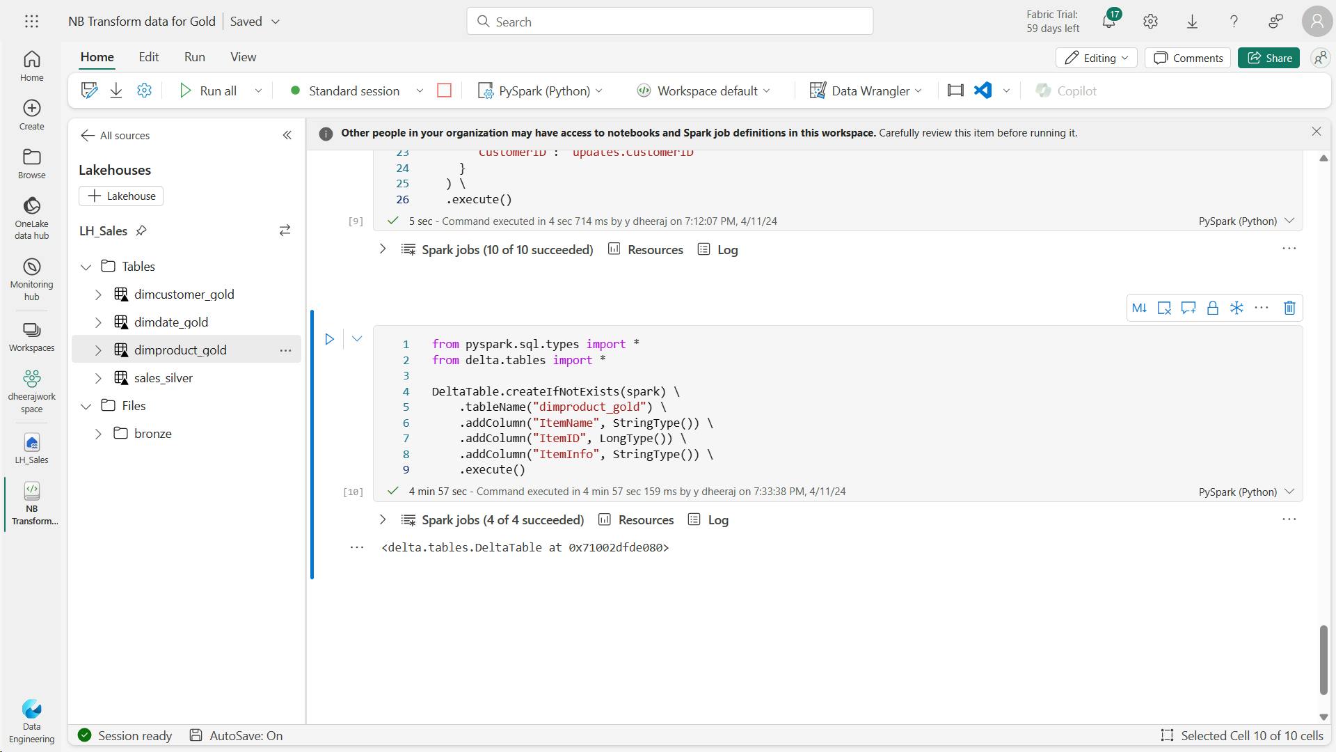
j. Code to to create the product_silver dataframe
from pyspark.sql.functions import col, split, lit

# Create product_silver dataframe

dfdimProduct_silver = df.dropDuplicates(["Item"]).select(col("Item")) \
    .withColumn("ItemName",split(col("Item"), ", ").getItem(0)) \
    .withColumn("ItemInfo",when((split(col("Item"), ", ").getItem(1).isNull() | (split(col("Item"), ", ").getItem(1)=="")),lit("")).otherwise(split(col("Item"), ", ").getItem(1)))

# Display the first 10 rows of the dataframe to preview your data

display(dfdimProduct_silver.head(10))
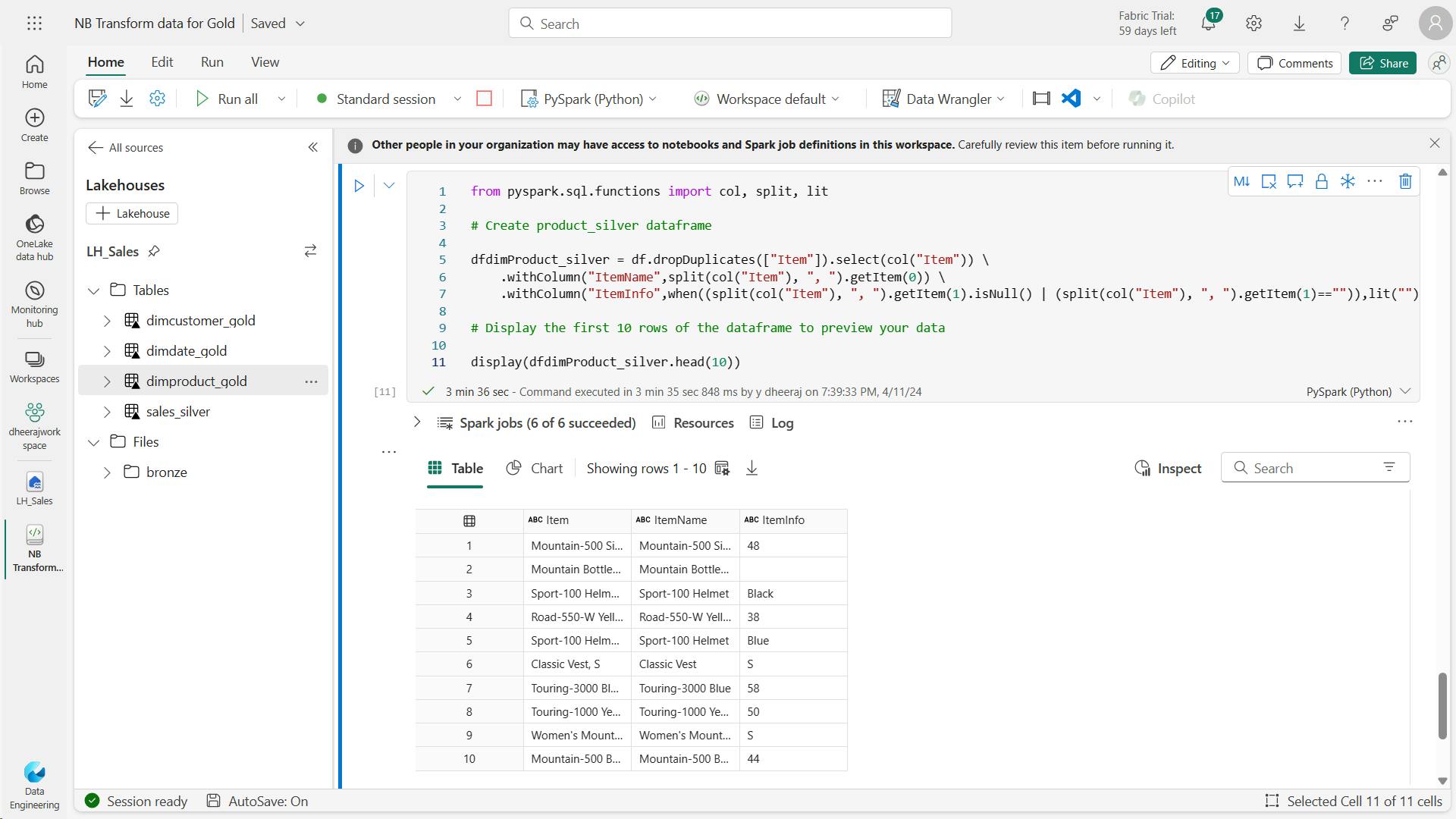
k. Code to create IDs for your dimProduct_gold table
This calculates the next available product ID based on the current data in the table, assigns these new IDs to the products, and then displays the updated product information.
from pyspark.sql.functions import monotonically_increasing_id, col, lit, max, coalesce

#dfdimProduct_temp = dfdimProduct_silver
dfdimProduct_temp = spark.read.table("dimproduct_gold")

MAXProductID = dfdimProduct_temp.select(coalesce(max(col("ItemID")),lit(0)).alias("MAXItemID")).first()[0]

dfdimProduct_gold = dfdimProduct_silver.join(dfdimProduct_temp,(dfdimProduct_silver.ItemName == dfdimProduct_temp.ItemName) & (dfdimProduct_silver.ItemInfo == dfdimProduct_temp.ItemInfo), "left_anti")

dfdimProduct_gold = dfdimProduct_gold.withColumn("ItemID",monotonically_increasing_id() + MAXProductID + 1)

# Display the first 10 rows of the dataframe to preview your data

display(dfdimProduct_gold.head(10))
from her
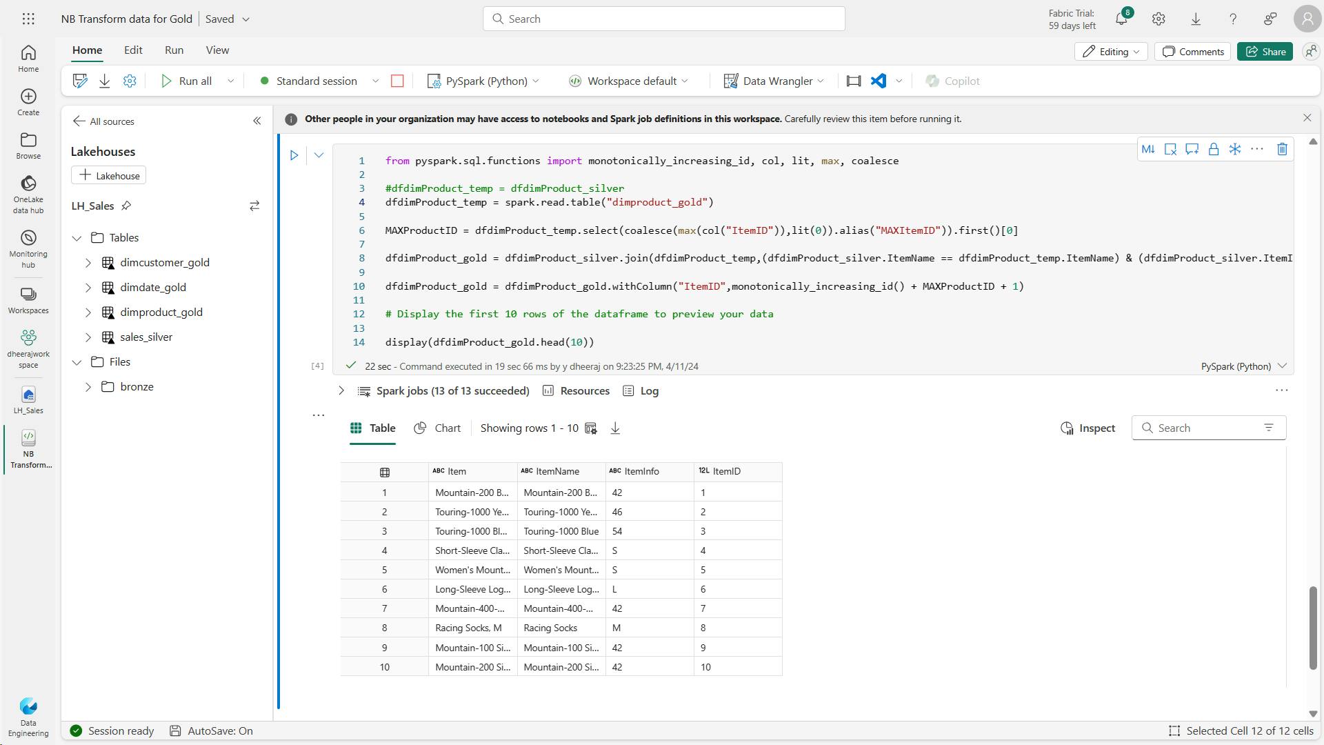
l. Code to ensure that your product table remains up-to-date as new data comes in
from delta.tables import *

deltaTable = DeltaTable.forPath(spark, 'Tables/dimproduct_gold')

dfUpdates = dfdimProduct_gold

deltaTable.alias('silver') \
  .merge(
        dfUpdates.alias('updates'),
        'silver.ItemName = updates.ItemName AND silver.ItemInfo = updates.ItemInfo'
        ) \
        .whenMatchedUpdate(set =
        {

        }
        ) \
        .whenNotMatchedInsert(values =
         {
          "ItemName": "updates.ItemName",
          "ItemInfo": "updates.ItemInfo",
          "ItemID": "updates.ItemID"
          }
          ) \
          .execute()
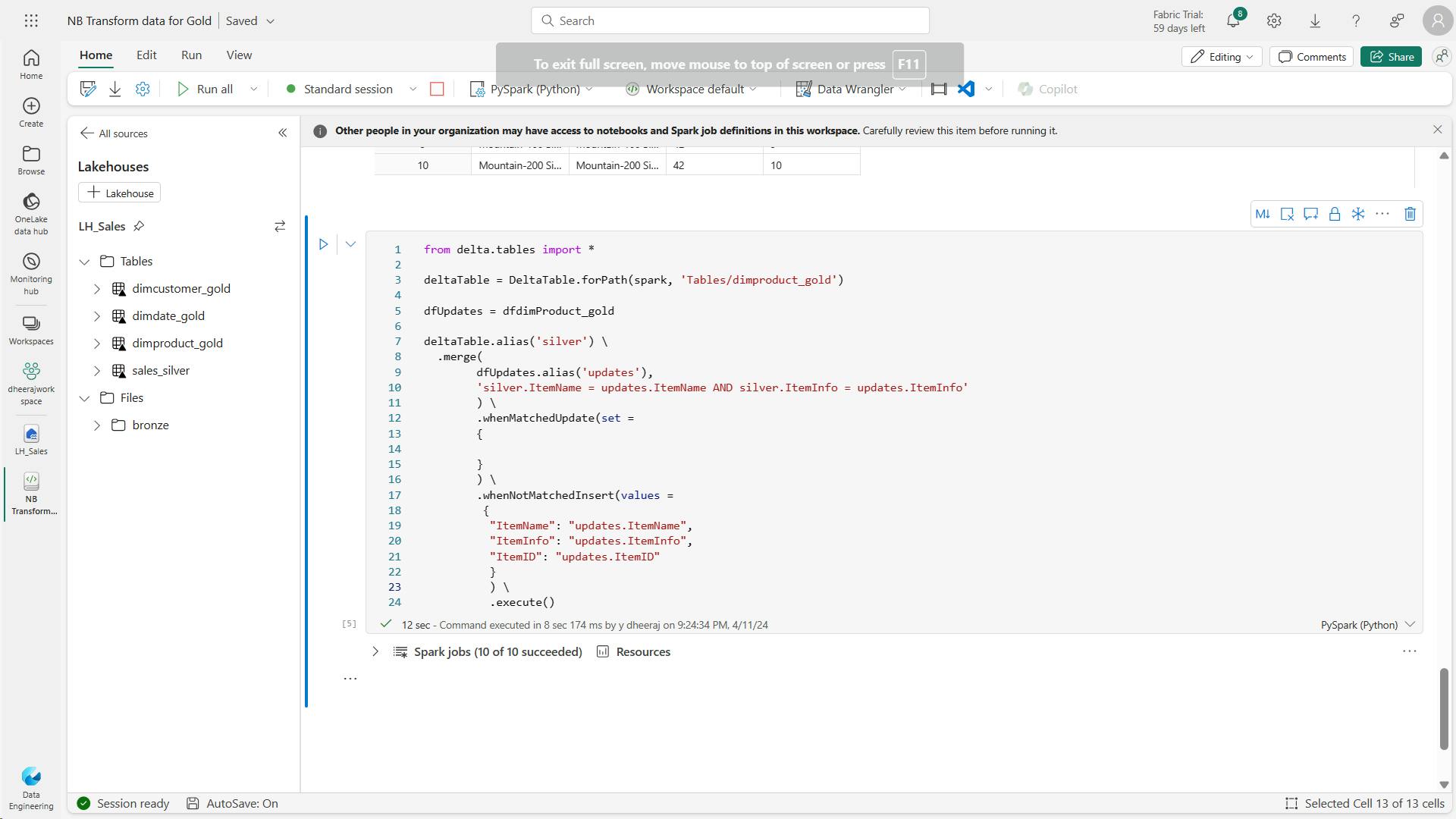
Refresh LH
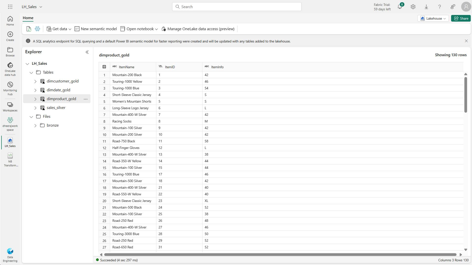
Fact table:
m. Code to create the fact table
from pyspark.sql.types import *
from delta.tables import *

DeltaTable.createIfNotExists(spark) \
    .tableName("factsales_gold") \
    .addColumn("CustomerID", LongType()) \
    .addColumn("ItemID", LongType()) \
    .addColumn("OrderDate", DateType()) \
    .addColumn("Quantity", IntegerType()) \
    .addColumn("UnitPrice", FloatType()) \
    .addColumn("Tax", FloatType()) \
    .execute()
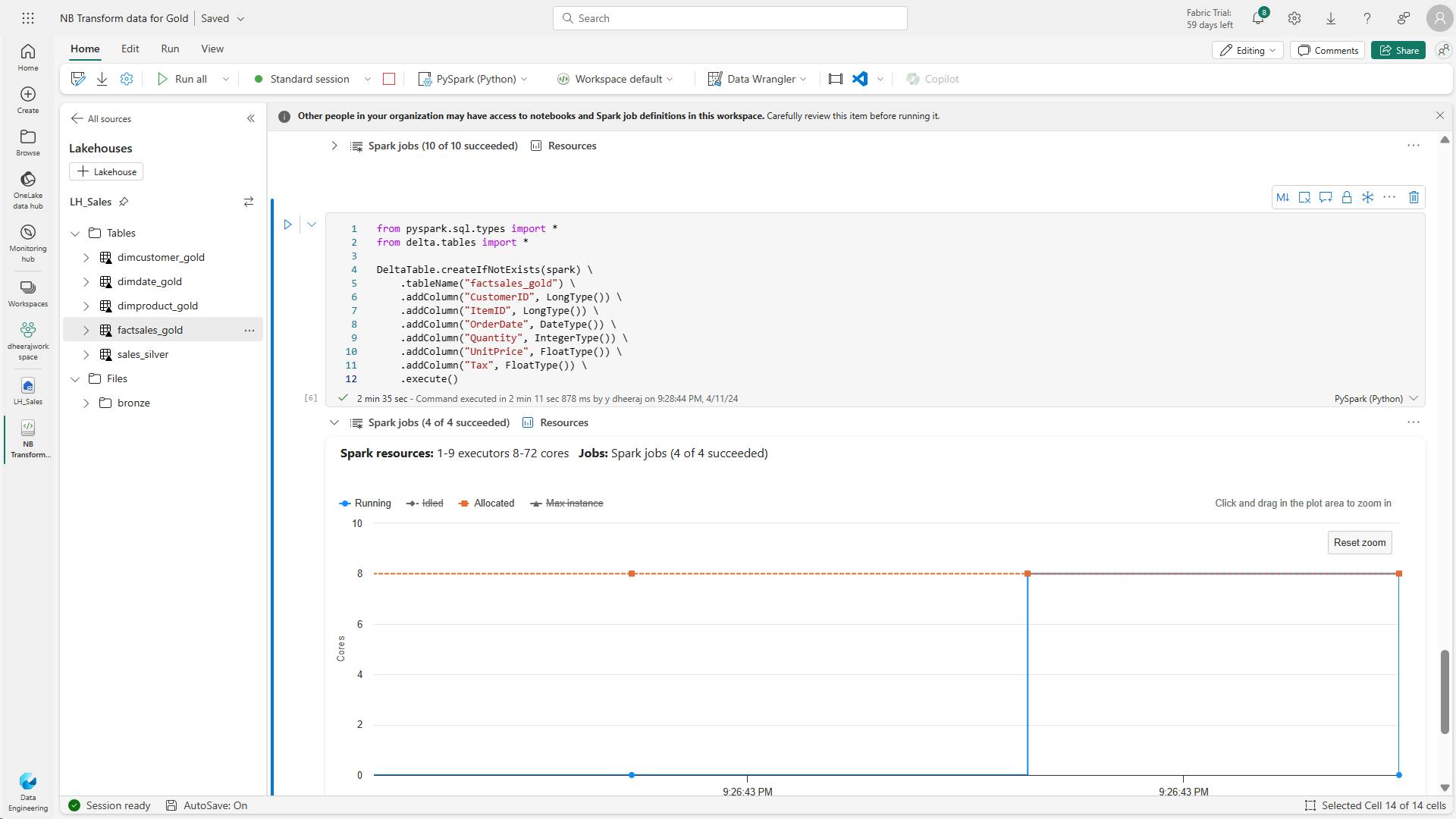
n. Code to create a new dataframe to combine sales data with customer and product information include customer ID, item ID, order date, quantity, unit price, and tax
from pyspark.sql.functions import col, split, when, lit

dfdimCustomer_temp = spark.read.table("dimcustomer_gold")
dfdimProduct_temp = spark.read.table("dimproduct_gold")

df = df.withColumn("ItemName",split(col("Item"), ", ").getItem(0)) \
    .withColumn("ItemInfo",when((split(col("Item"), ", ").getItem(1).isNull() | (split(col("Item"), ", ").getItem(1)=="")),lit("")).otherwise(split(col("Item"), ", ").getItem(1))) \


# Create Sales_gold dataframe

dffactSales_gold = df.alias("df1").join(dfdimCustomer_temp.alias("df2"),(df.CustomerName == dfdimCustomer_temp.CustomerName) & (df.Email == dfdimCustomer_temp.Email), "left") \
        .join(dfdimProduct_temp.alias("df3"),(df.ItemName == dfdimProduct_temp.ItemName) & (df.ItemInfo == dfdimProduct_temp.ItemInfo), "left") \
    .select(col("df2.CustomerID") \
        , col("df3.ItemID") \
        , col("df1.OrderDate") \
        , col("df1.Quantity") \
        , col("df1.UnitPrice") \
        , col("df1.Tax") \
    ).orderBy(col("df1.OrderDate"), col("df2.CustomerID"), col("df3.ItemID"))

# Display the first 10 rows of the dataframe to preview your data

display(dffactSales_gold.head(10))
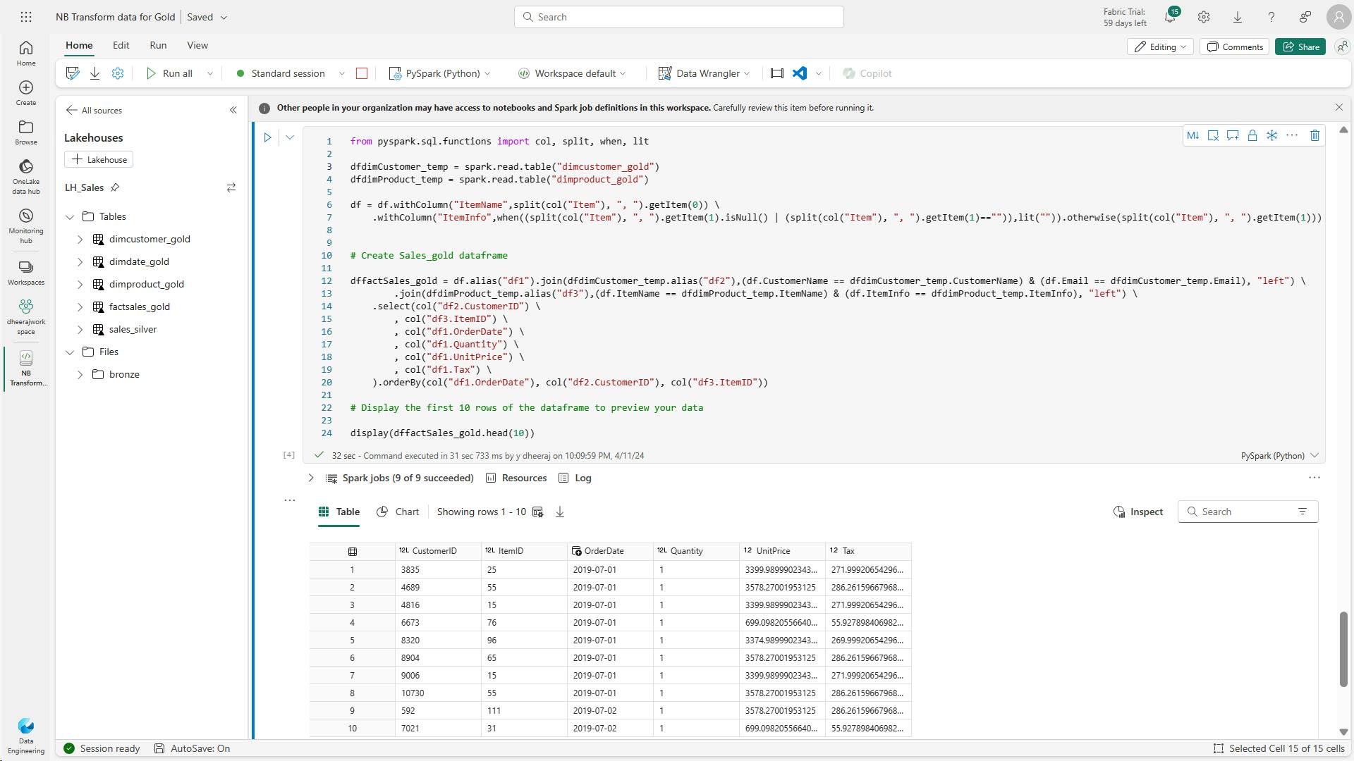
o. Code to ensure that sales data remains up-to-date
Here you’re using Delta Lake’s merge operation to synchronize and update the factsales_gold table with new sales data (dffactSales_gold).
The operation compares the order date, customer ID, and item ID between the existing data (silver table) and the new data (updates DataFrame), updating matching records and inserting new records as needed.
from delta.tables import *

deltaTable = DeltaTable.forPath(spark, 'Tables/factsales_gold')

dfUpdates = dffactSales_gold

deltaTable.alias('silver') \
  .merge(
    dfUpdates.alias('updates'),
    'silver.OrderDate = updates.OrderDate AND silver.CustomerID = updates.CustomerID AND silver.ItemID = updates.ItemID'
  ) \
   .whenMatchedUpdate(set =
    {

    }
  ) \
 .whenNotMatchedInsert(values =
    {
      "CustomerID": "updates.CustomerID",
      "ItemID": "updates.ItemID",
      "OrderDate": "updates.OrderDate",
      "Quantity": "updates.Quantity",
      "UnitPrice": "updates.UnitPrice",
      "Tax": "updates.Tax"
    }
  ) \
  .execute()

You now have a curated, modeled gold layer that can be used for reporting and analysis.
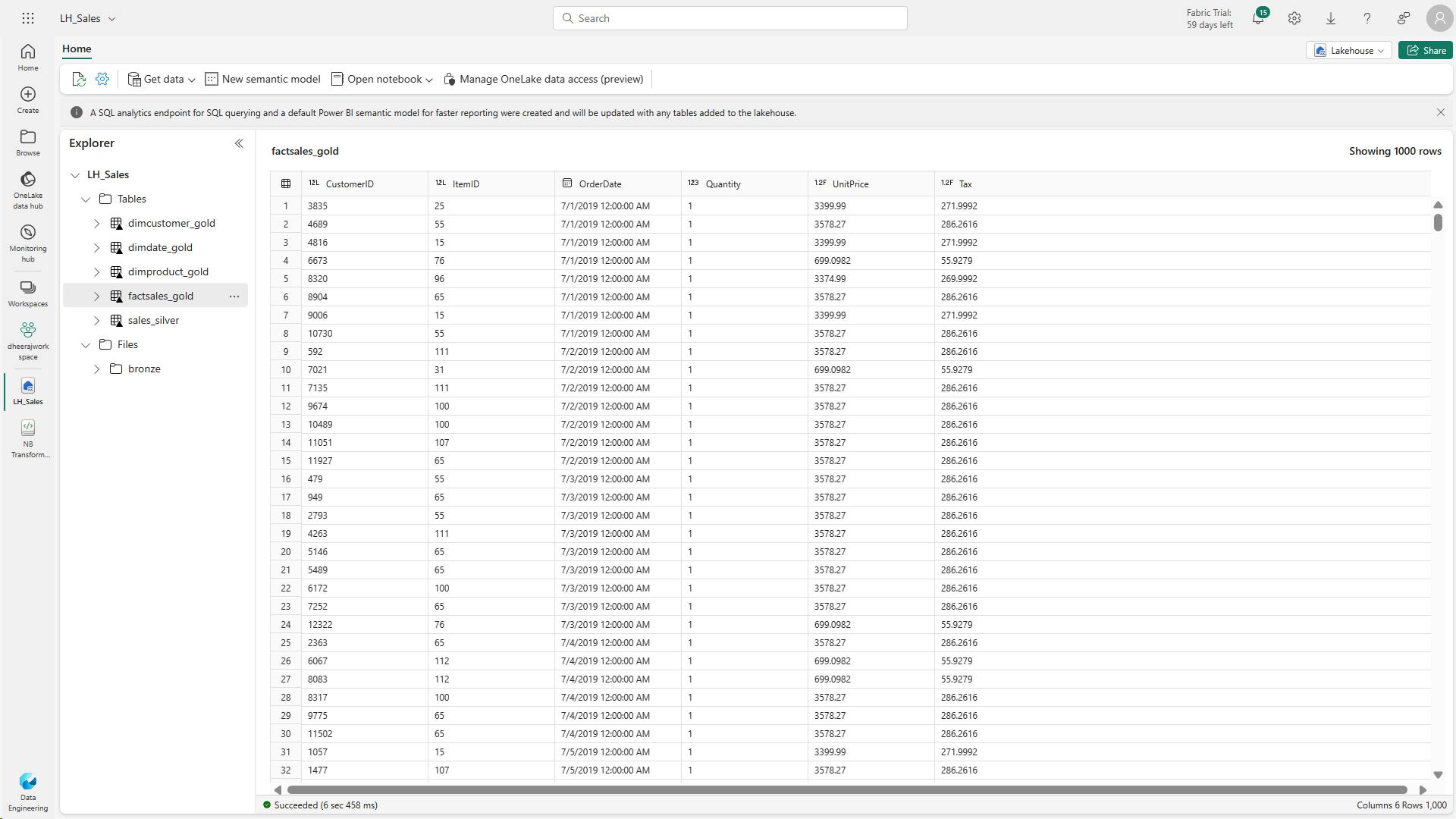
vi. Create a semantic model
In your workspace, you can now use the gold layer to create a report and analyze the data.
You can access the semantic model directly in your workspace to create relationships and measures for reporting.
Note that you can’t use the default semantic model that is automatically created when you create a lakehouse.
You must create a new semantic model that includes the gold tables you created in this exercise, from the lakehouse explorer.
Error:
Unexpected error dispatching create semantic model to portal action handler
Sales_Gold to your new semantic model.
From here, you or other members of your data team can create reports and dashboards based on the data in your lakehouse.
These reports will be connected directly to the gold layer of your lakehouse, so they’ll always reflect the latest data.
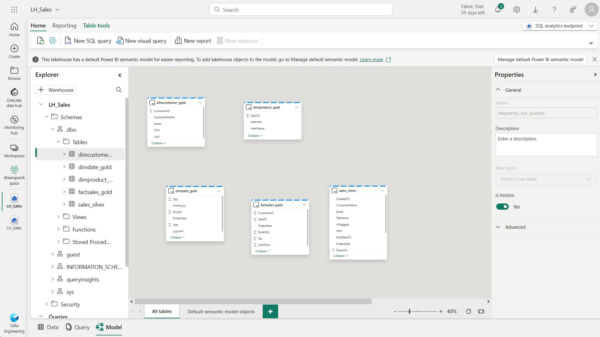
vii. Clean up resources
you’ve learned how to create a medallion architecture in a Microsoft Fabric lakehouse.
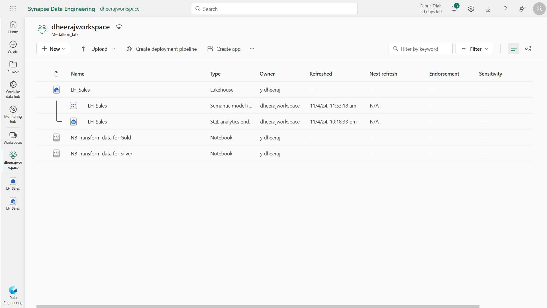
7. Knowledge check
Which of the following sets of layers are typically associated with the Medallion Architecture for data management?
Bronze, Silver, Gold
Bronze, silver, gold is the correct sequence of layers typically used in the medallion architecture. Data flows from the raw and unrefined state (bronze) to a curated and validated state (silver), and finally to an enriched and well-structured presentation state (gold).
Which tool is best suited for data transformation in Fabric when dealing with large-scale data that will continue to grow?
Notebooks
Notebooks are a more suitable tool for data transformation with big data in Fabric.
What is the benefit of storing different layers of your lakehouse in separate workspaces?
Storing different layers of your lakehouse in separate workspaces enhances security and optimizes cost-effectiveness.
8. Summary
You now understand how the medallion architecture offers a structured approach to logically organize lakehouse data. Once you integrate this architecture into your Fabric setup, you're on your way to ensuring an organized, refined, and curated data system.
You'll eliminate data silos and ensure that downstream teams and apps can access and use the data seamlessly. With this effective setup, you're not just storing data; you're setting it up to be quickly and easily analyzed by whenever it's needed.
Learning objectives
In this module, you'll learn how to:
Describe the principles of using the medallion architecture in data management.
Apply the medallion architecture framework within the Microsoft Fabric environment.
Analyze data stored in the lakehouse using DirectLake in Power BI.
Describe best practices for ensuring the security and governance of data stored in the medallion architecture.
IX. Get started with data warehouses in Microsoft Fabric
Data warehouses are analytical stores built on a relational schema to support SQL queries.
Microsoft Fabric enables you to create a relational data warehouse in your workspace and integrate it easily with other elements of your end-to-end analytics solution.
1. Introduction
Relational data warehouses are at the center of most enterprise business intelligence (BI) solutions.
While the specific details may vary across data warehouse implementations, a common pattern based on a denormalized, multidimensional schema has emerged as the standard design for a relational data warehouse.
Microsoft Fabric's data warehouse is a modern version of the traditional data warehouse.
It centralizes and organizes data from different departments, systems, and databases into a single, unified view for analysis and reporting purposes.
Fabric's data warehouse provides full SQL semantics, including the ability to insert, update, and delete data in the tables.
Fabric's data warehouse is unique because it's built on the Lakehouse, which is stored in Delta format and can be queried using SQL. It's designed for use by the whole data team, not just data engineers.
Fabric's data warehouse experience is designed to address these challenges. Fabric enables data engineers, analysts, and data scientists to work together to create and query a data warehouse that is optimized for their specific needs.
In this module, you'll learn about data warehouses in Fabric, create a data warehouse, load, query, and visualize data.
2. Understand data warehouse fundamentals
The process of building a modern data warehouse typically consists of:
Data ingestion - moving data from source systems into a data warehouse.
Data storage - storing the data in a format that is optimized for analytics.
Data processing - transforming the data into a format that is ready for consumption by analytical tools.
Data analysis and delivery - analyzing the data to gain insights and delivering those insights to the business.
Microsoft Fabric enables data engineers and analysts to ingest, store, transform, and visualize data all in one tool with both a low-code and traditional experience.
i. Understand Fabric's data warehouse experience
Fabric's data warehouse is a relational data warehouse that supports the full transactional T-SQL capabilities you'd expect from an enterprise data warehouse.
It's a fully managed, scalable, and highly available data warehouse that can be used to store and query data in the Lakehouse.
Using the data warehouse, you're fully in control of creating tables, loading, transforming, and querying data using either the Fabric portal or T-SQL commands. You can use SQL to query and analyze the data, or use Spark to process the data and create machine learning models.
Data warehouses in Fabric facilitate collaboration between data engineers and data analysts, working together in the same experience. Data engineers build a relational layer on top of data in the Lakehouse, where analysts can use T-SQL and Power BI to explore the data.
ii. Design a data warehouse
Like all relational databases, Fabric's data warehouse contains tables to store your data for analytics later.
Most commonly, these tables are organized in a schema that is optimized for multidimensional modeling. In this approach, numerical data related to events (e.g. sales orders) are grouped by different attributes (e.g. date, customer, store).
For instance, you can analyze the total amount paid for sales orders that occurred on a specific date or at a particular store.
a. Tables in a data warehouse (fact tables and dimension tables)
Tables in a data warehouse are typically organized in a way that supports efficient and effective analysis of large amounts of data.
This way of organizing tables is often referred to as dimensional modeling, which involves structuring tables into fact tables and dimension tables.
1. Fact tables
Fact tables contain the numerical data that you want to analyze. Fact tables typically have a large number of rows and are the primary source of data for analysis.
For example, a fact table might contain the total amount paid for sales orders that occurred on a specific date or at a particular store.
2. Dimension tables
Dimension tables contain descriptive information about the data in the fact tables.
Dimension tables typically have a small number of rows and are used to provide context for the data in the fact tables.
For example, a dimension table might contain information about the customers who placed sales orders.
In addition to attribute columns, a dimension table contains a unique key column that uniquely identifies each row in the table.
In fact, it's common for a dimension table to include two key columns:
A surrogate key is a unique identifier for each row in the dimension table. It's often an integer value that is automatically generated by the database management system when a new row is inserted into the table.
An alternate key is often a natural or business key that identifies a specific instance of an entity in the transactional source system - such as a product code or a customer ID.
You need both surrogate and alternate keys in a data warehouse, because they serve different purposes.
Surrogate keys are specific to the data warehouse and help to maintain consistency and accuracy in the data.
Alternate keys on the other hand are specific to the source system and help to maintain traceability between the data warehouse and the source system.
b. Special types of dimension tables
Special types of dimensions provide additional context and enable more comprehensive data analysis.
Time dimensions provide information about the time period in which an event occurred. This table enables data analysts to aggregate data over temporal intervals. For example, a time dimension might include columns for the year, quarter, month, and day in which a sales order was placed.
Slowly changing dimensions are dimension tables that track changes to dimension attributes over time, like changes to a customer's address or a product's price. They're significant in a data warehouse because they enable users to analyze and understand changes to data over time. Slowly changing dimensions ensure that data stays up-to-date and accurate, which is imperative to making good business decisions.
ii. Data warehouse schema designs
In most transactional databases that are used in business applications, the data is normalized to reduce duplication. In a data warehouse however, the dimension data is generally de-normalized to reduce the number of joins required to query the data.
Often, a data warehouse is organized as a star schema, in which a fact table is directly related to the dimension tables, as shown in this example:
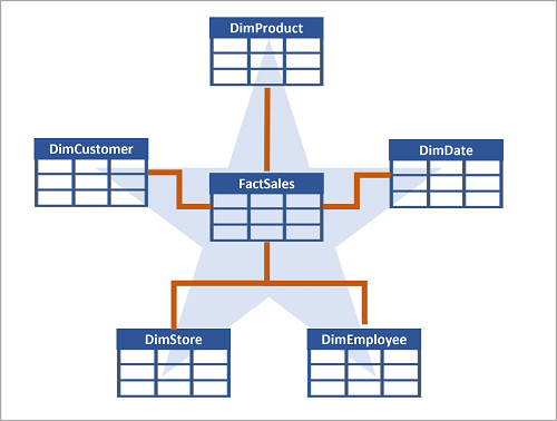
You can use the attributes of something to group together numbers in the fact table at different levels.
For example, you could find the total sales revenue for a whole region or just for one customer. The information for each level can be stored in the same dimension table.
If there are lots of levels or some information is shared by different things, it might make sense to use a snowflake schema instead. Here's an example:
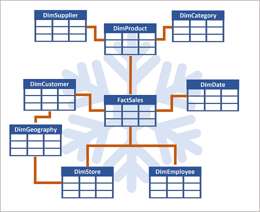
In this case, the DimProduct table has been split up (normalized) to create separate dimension tables for product categories and suppliers.
Each row in the DimProduct table contains key values for the corresponding rows in the DimCategory and DimSupplier tables. A DimGeography table has been added containing information on where customers and stores are located.
Each row in the DimCustomer and DimStore tables contains a key value for the corresponding row in the DimGeography table.
3. Understand data warehouses in Fabric
Fabric's Lakehouse is a collection of files, folders, tables, and shortcuts that act like a database over a data lake.
It's used by the Spark engine and SQL engine for big data processing and has features for ACID transactions when using the open-source Delta formatted tables.
The Lakehouse is a great place to store data, but it's not the best place to serve data to business users.
For that, you need a data warehouse.
Fabric's data warehouse experience allows you to transition from the lake view of the Lakehouse (which supports data engineering and Apache Spark) to the SQL experiences that a traditional data warehouse would provide.
The Lakehouse gives you the ability to read tables and use the SQL analytics endpoint, whereas the data warehouse enables you to manipulate the data.
In the data warehouse experience, you'll model data using tables and views, run T-SQL to query data across the data warehouse and Lakehouse, use T-SQL to perform DML operations on data inside the data warehouse, and serve reporting layers like Power BI.
Now that you understand the basic architectural principles for a relational data warehouse schema, let's explore how to create a data warehouse.
i. Describe a data warehouse in Fabric
In the data warehouse experience in Fabric, you can build a relational layer on top of physical data in the Lakehouse and expose it to analysis and reporting tools.
You can create your data warehouse directly in Fabric from the create hub or within a workspace. After creating an empty warehouse, you can add objects to it.
Once your warehouse is created, you can create tables using T-SQL directly in the Fabric interface.
ii. Ingest data into your data warehouse
There are a few ways to ingest data into a Fabric data warehouse, including Pipelines, Dataflows, cross-database querying, and the COPY INTO command.
After ingestion, the data becomes available for analysis by multiple business groups, who can use features such as cross-database querying and sharing to access it.
a. Create tables
To create a table in the data warehouse, you can use SQL Server Management Studio (SSMS) or another SQL client to connect to the data warehouse and run a CREATE TABLE statement.
You can also create tables directly in the Fabric UI.
You can copy data from an external location into a table in the data warehouse using the COPY INTO syntax.
COPY INTO dbo.Region
FROM 'https://mystorageaccountxxx.blob.core.windows.net/private/Region.csv' WITH (
            FILE_TYPE = 'CSV'
            ,CREDENTIAL = (
                IDENTITY = 'Shared Access Signature'
                , SECRET = 'xxx'
                )
            ,FIRSTROW = 2
            )
GO
This SQL query loads data from a CSV file stored in Azure Blob Storage into a table called "Region" in the Fabric data warehouse.
b. Table considerations
After creating tables in a data warehouse, it's important to consider the process of loading data into those tables. A common approach is to use staging tables. In Fabric, you can use T-SQL commands to load data from files into staging tables in the data warehouse.
Staging tables are temporary tables that can be used to perform data cleansing, data transformations, and data validation. You can also use staging tables to load data from multiple sources into a single destination table.
Usually, data loading is performed as a periodic batch process in which inserts and updates to the data warehouse are coordinated to occur at a regular interval (for example, daily, weekly, or monthly).
Generally, you should implement a data warehouse load process that performs tasks in the following order:
Ingest the new data to be loaded into a data lake, applying pre-load cleansing or transformations as required.
Load the data from files into staging tables in the relational data warehouse.
Load the dimension tables from the dimension data in the staging tables, updating existing rows or inserting new rows and generating surrogate key values as necessary.
Load the fact tables from the fact data in the staging tables, looking up the appropriate surrogate keys for related dimensions.
Perform post-load optimization by updating indexes and table distribution statistics.
If you have tables in the lakehouse, and you want to be able to query it in your warehouse - but not make changes -
With a Fabric data warehouse, you don't have to copy data from the lakehouse to the data warehouse. You can query data in the lakehouse directly from the data warehouse using cross-database querying.
4. Query and transform data
Now that you know how to implement a data warehouse in Fabric, let's prepare the data for analytics.
There are two ways to query data from your data warehouse. The Visual query editor provides a no-code, drag-and-drop experience to create your queries. If you're comfortable with T-SQL, you may prefer to use the SQL query editor to write your queries. In both cases, you can create tables, views, and stored procedures to query data in the data warehouse and Lakehouse.
There's also a SQL analytics endpoint, where you can connect from any tool.
i. Query data using the SQL query editor
ii. Query data using the Visual query editor
5. Prepare data for analysis and reporting
A semantic model defines the relationships between the different tables in the semantic model, the rules for how data is aggregated and summarized, and the calculations or measures that are used to derive insights from the data.
These relationships and measures are included in the semantic model, which is then used to create reports in Power BI.
i. Build relationships
ii. Create measures
Measures are the metrics that you want to analyze in your data warehouse.
Measures are calculated fields that are based on the data in the tables in your data warehouse using the Data Analysis Expressions (DAX) formula language.
iii. Hide fields
iv. Understand semantic models
Every time a data warehouse is created, Fabric creates a semantic model for analysts and/or business users to connect to for reporting.
Semantic model has metrics that are used to create reports. Simply put, analysts use the semantic model you created in your warehouse, which is stored in a semantic model.
Semantic models are automatically kept in sync with the data warehouse, so you don't have to worry about maintaining them. You can also create custom semantic models to meet your specific needs.
v. Understand the default semantic model
There's also a default semantic model automatically created for you in Fabric.
It inherits business logic from the parent lakehouse or warehouse, which initiates the downstream analytics experience for business intelligence and analysis.
This semantic model is managed, optimized, and kept in sync for you.
vi. Visualize data
6. Secure and monitor your data warehouse
i. Security
Data warehouse security is important to protect your data from unauthorized access.
Fabric provides a number of security features to help you secure your data warehouse.
These include:
Role-based access control (RBAC) to control access to the warehouse and its data.
SSL encryption to secure the communication between the warehouse and the client applications.
Azure Storage Service Encryption to protect the data in transit and at rest.
Azure Monitor and Azure Log Analytics to monitor the warehouse activity and audit the access to the data.
Multifactor authentication (MFA) to add an extra layer of security to user accounts.
Microsoft Entra ID integration to manage the user identities and access to the warehouse.
ii. Workspace permissions
Appropriate workspace roles are the first line of defense in securing your data warehouse.
In addition to workspace roles, you can grant item permissions and access through SQL.
iii. Item permissions
You can grant permissions to users via T-SQL or in the Fabric portal. Grant the following permissions to users who need to access your data warehouse:
Read: Allows the user to CONNECT using the SQL connection string.
ReadData: Allows the user to read data from any table/view within the warehouse.
ReadAll: Allows user to read data the raw parquet files in OneLake that can be consumed by Spark.
A user connection to the SQL analytics endpoint will fail without Read permission at a minimum.
iv. Monitoring
Monitoring activities in your data warehouse is crucial to ensure optimal performance, efficient resource utilization, and security. It helps you identify issues, detect anomalies, and take action to keep the data warehouse running smoothly and securely.
You can use dynamic management views (DMVs) to monitor connection, session, and request status to see live SQL query lifecycle insights. With DMVs, you can get details like the number of active queries and identify which queries are running for an extended period and require termination.
There are currently three DMVs available to use in Fabric:
sys.dm_exec_connections: Returns information about each connection established between the warehouse and the engine.
sys.dm_exec_sessions: Returns information about each session authenticated between the item and engine.
sys.dm_exec_requests: Returns information about each active request in a session.
v. Query monitoring
Use 'sys.dm_exec_requests' to identify long-running queries that may be impacting the overall performance of the database, and take appropriate action to optimize or terminate those queries.
Start by identifying the queries that have been running for a long time. Use the following query to identify which queries have been running the longest, in descending order:
SELECT request_id, session_id, start_time, total_elapsed_time
FROM sys.dm_exec_requests
WHERE status = 'running'
ORDER BY total_elapsed_time DESC;
You can continue investigating to understand which user ran the session with the long-running query, by running:
SELECT login_name
FROM sys.dm_exec_sessions
WHERE 'session_id' = 'SESSION_ID WITH LONG-RUNNING QUERY';
use the KILL command to terminate the session with the long-running query:
KILL 'SESSION_ID WITH LONG-RUNNING QUERY';
Note:
You must be a workspace Admin to run the KILL command. Workspace Admins can execute all three DMVs.
Member role, Contributor role, and Viewer role can see their own results within the warehouse, but cannot see other users' results.
7. Exercise - Analyze data in a data warehouse
create a data warehouse in Fabric and analyze your data.
In Microsoft Fabric, a data warehouse provides a relational database for large-scale analytics.
Unlike the default read-only SQL endpoint for tables defined in a lakehouse, a data warehouse provides full SQL semantics; including the ability to insert, update, and delete data in the tables.
i. Create a workspace
ii. Create a data warehouse
iii. Create tables and insert data
A warehouse is a relational database in which you can define tables and other objects.
Create tables with T-SQL tile
CREATE TABLE statement
CREATE TABLE dbo.DimProduct
(
    ProductKey INTEGER NOT NULL,
    ProductAltKey VARCHAR(25) NULL,
    ProductName VARCHAR(50) NOT NULL,
    Category VARCHAR(50) NULL,
    ListPrice DECIMAL(5,2) NULL
);
GO
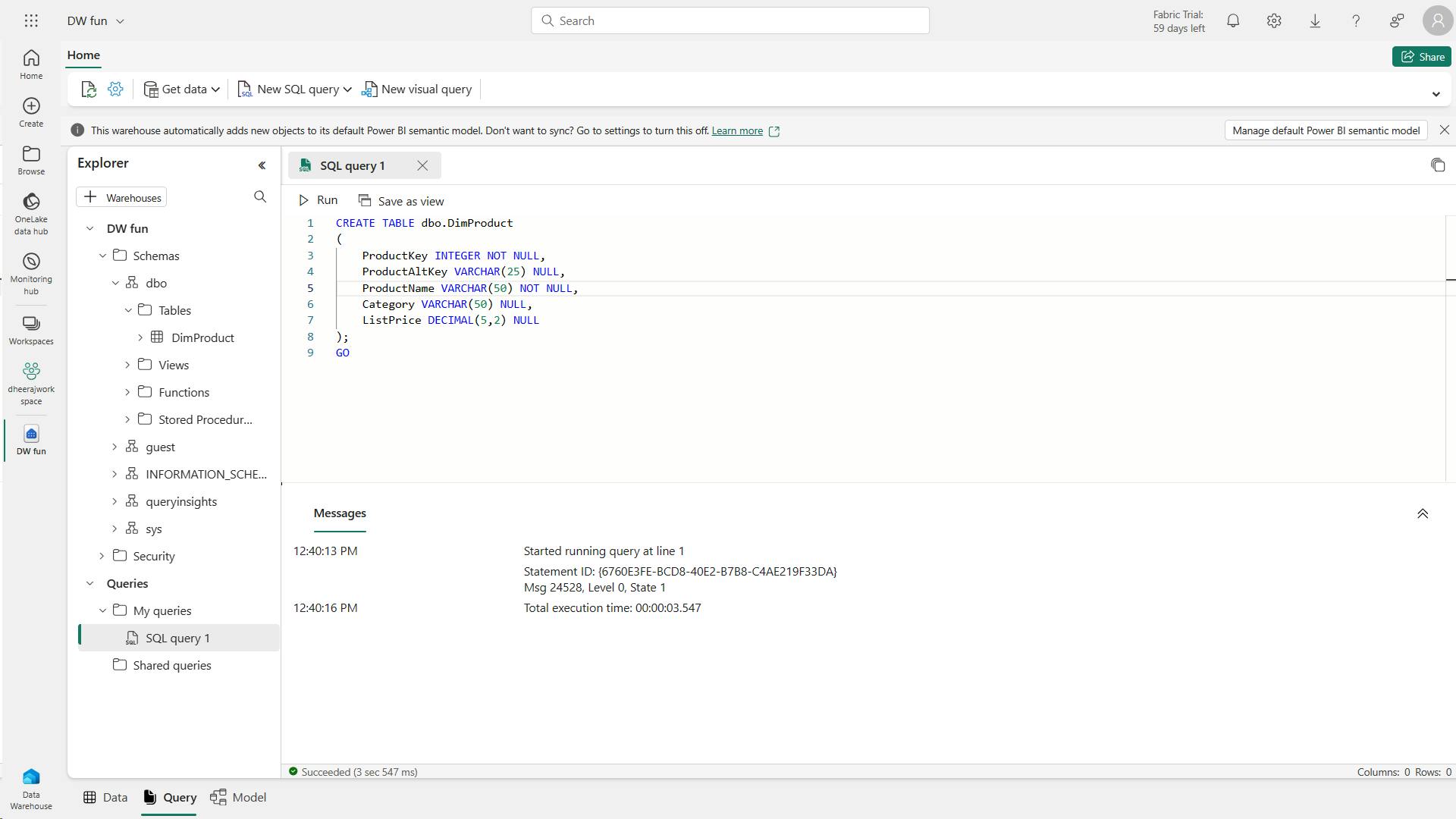
INSERT statement
INSERT INTO dbo.DimProduct
VALUES
(1, 'RING1', 'Bicycle bell', 'Accessories', 5.99),
(2, 'BRITE1', 'Front light', 'Accessories', 15.49),
(3, 'BRITE2', 'Rear light', 'Accessories', 15.49);
GO
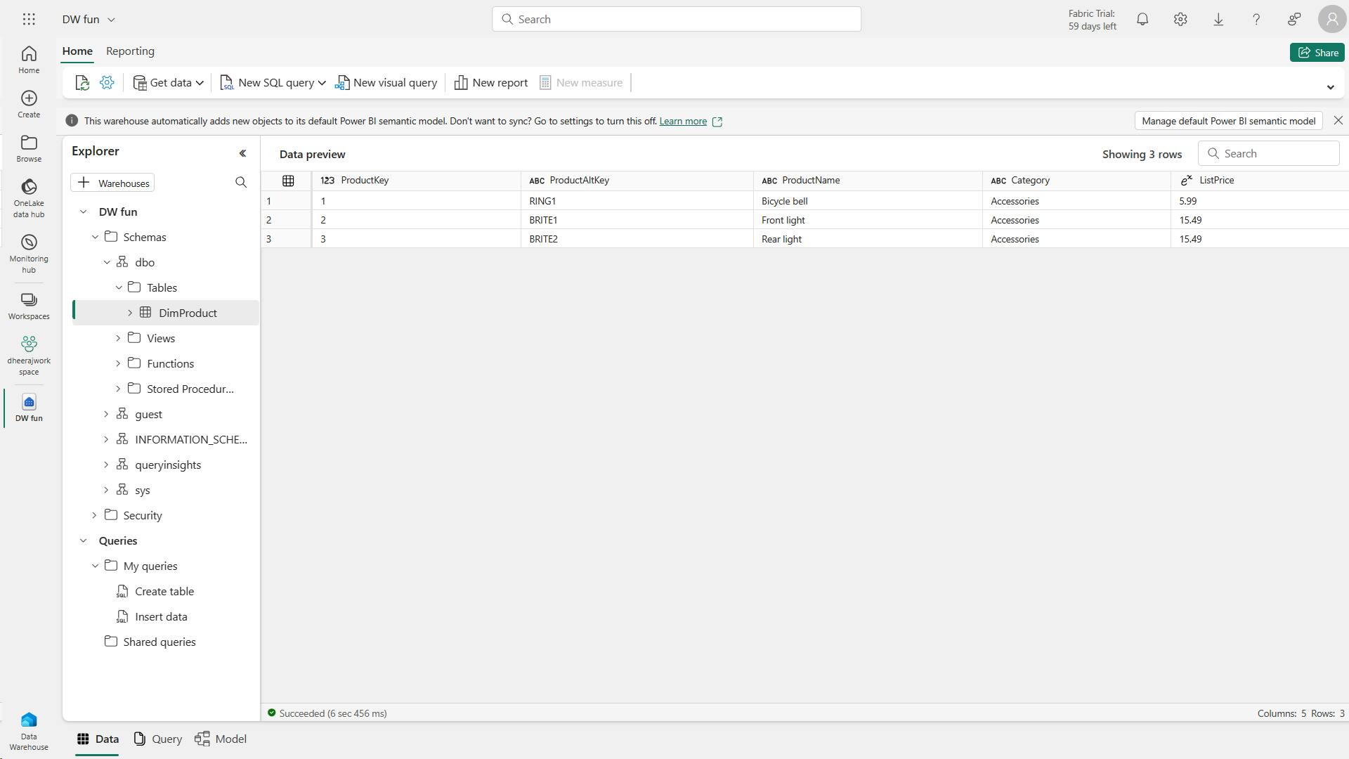
creates a simple data warehouse schema and loads some data
Data:
create-dw.txt [Link]
verify that the dbo schema in the data warehouse now contains the following four tables:
DimCustomer
DimDate
DimProduct
FactSalesOrder
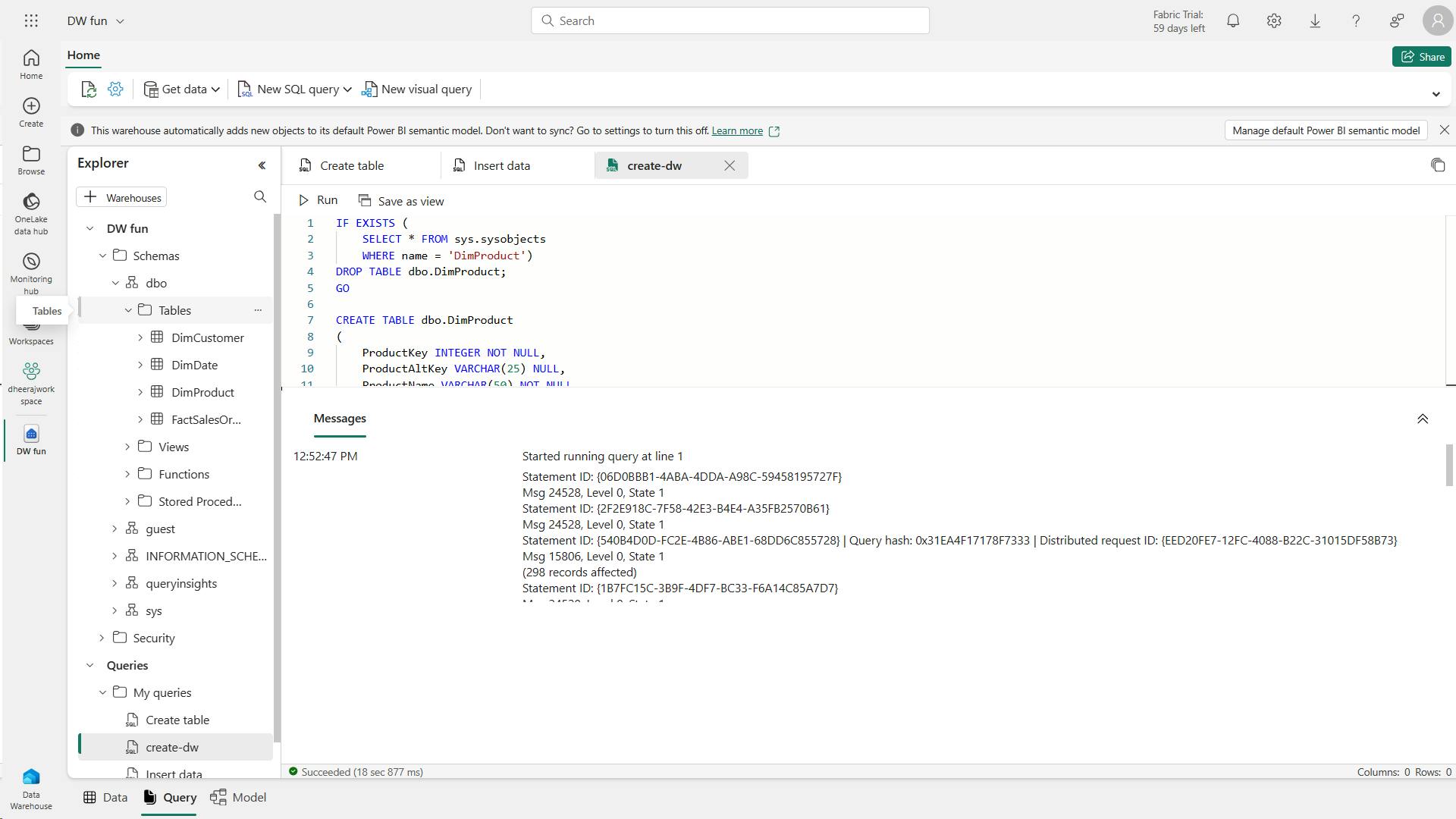
iv. Define a data model
A relational data warehouse typically consists of fact and dimension tables.
The fact tables contain numeric measures you can aggregate to analyze business performance (for example, sales revenue), and
The dimension tables contain attributes of the entities by which you can aggregate the data (for example, product, customer, or time).
In a Microsoft Fabric data warehouse, you can use these keys to define a data model that encapsulates the relationships between the tables.
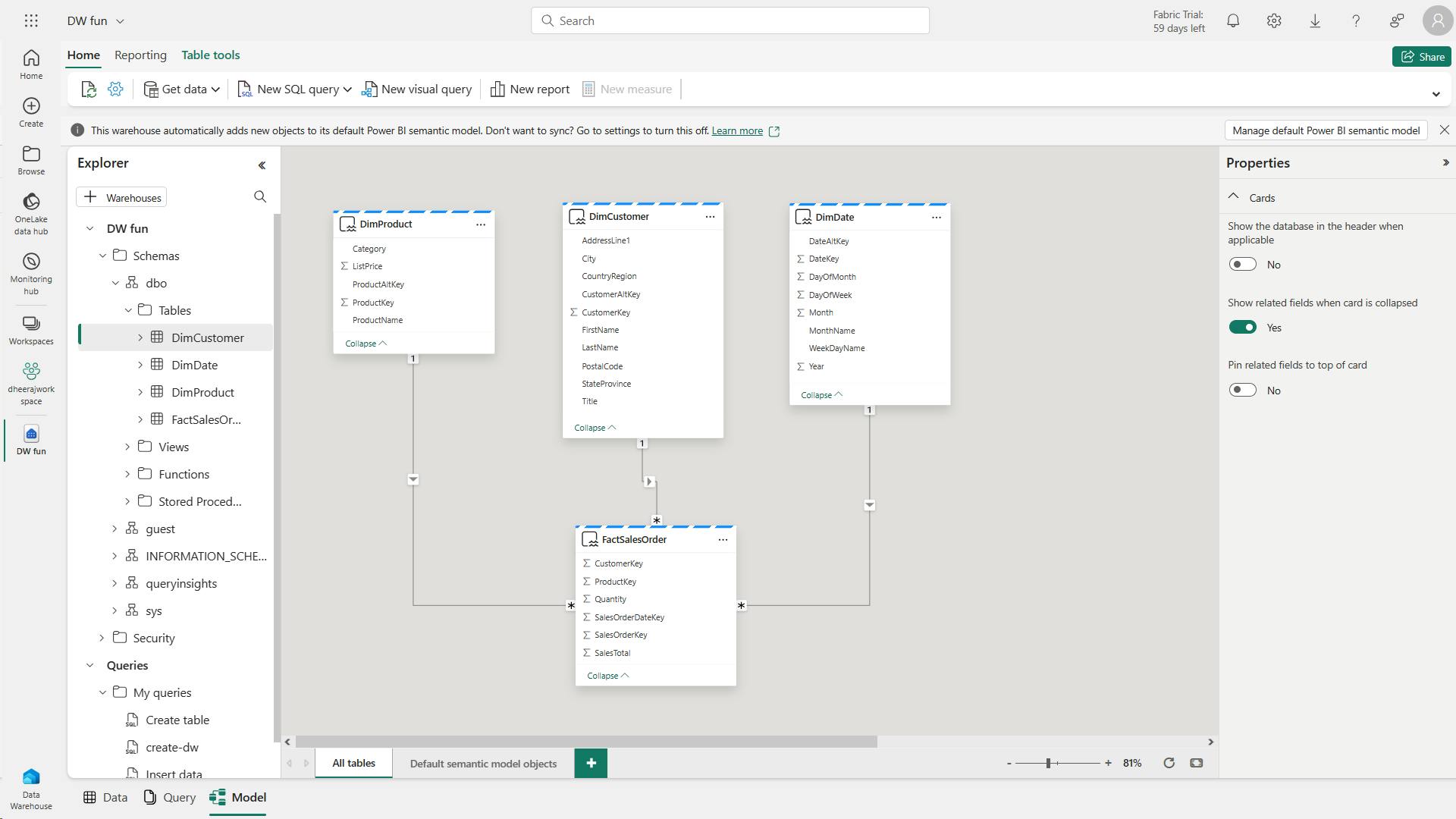
v. Query data warehouse tables
SELECT  d.[Year] AS CalendarYear,
         d.[Month] AS MonthOfYear,
         d.MonthName AS MonthName,
        SUM(so.SalesTotal) AS SalesRevenue
FROM FactSalesOrder AS so
JOIN DimDate AS d ON so.SalesOrderDateKey = d.DateKey
GROUP BY d.[Year], d.[Month], d.MonthName
ORDER BY CalendarYear, MonthOfYear;
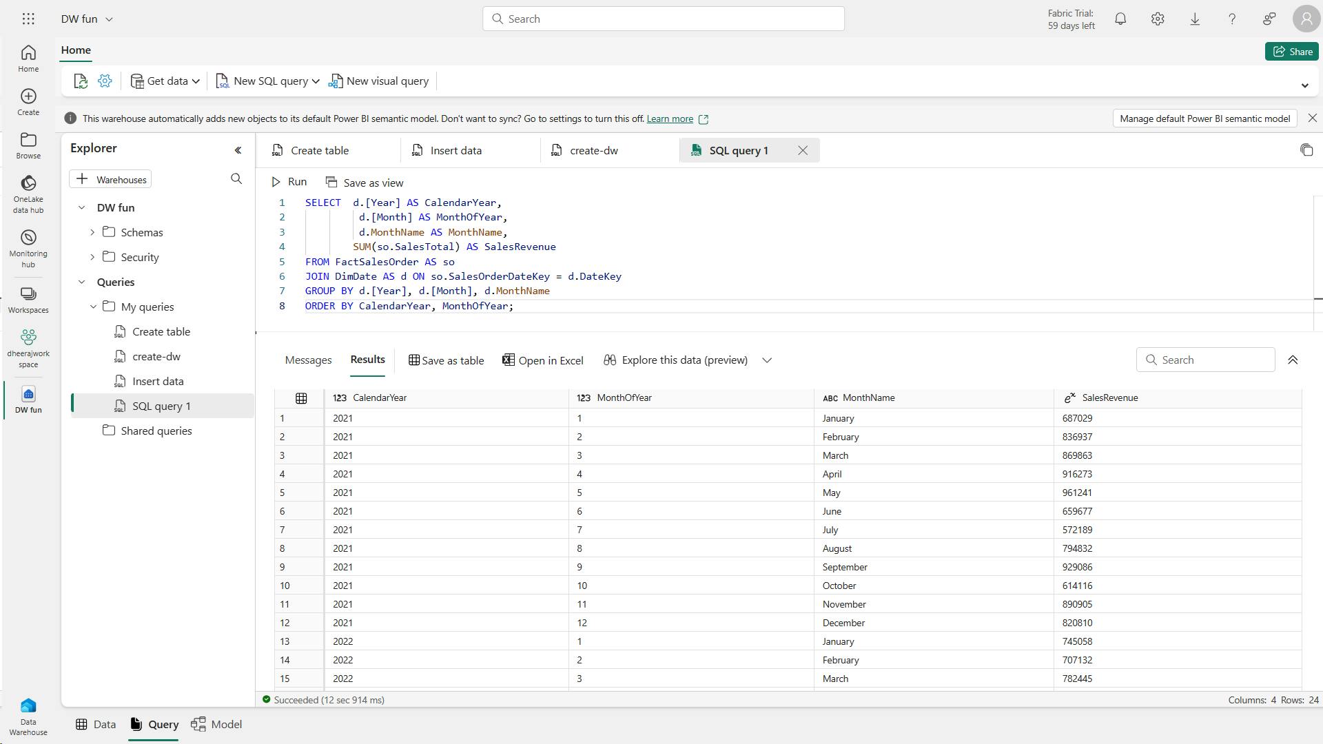
SELECT  d.[Year] AS CalendarYear,
        d.[Month] AS MonthOfYear,
        d.MonthName AS MonthName,
        c.CountryRegion AS SalesRegion,
       SUM(so.SalesTotal) AS SalesRevenue
FROM FactSalesOrder AS so
JOIN DimDate AS d ON so.SalesOrderDateKey = d.DateKey
JOIN DimCustomer AS c ON so.CustomerKey = c.CustomerKey
GROUP BY d.[Year], d.[Month], d.MonthName, c.CountryRegion
ORDER BY CalendarYear, MonthOfYear, SalesRegion;
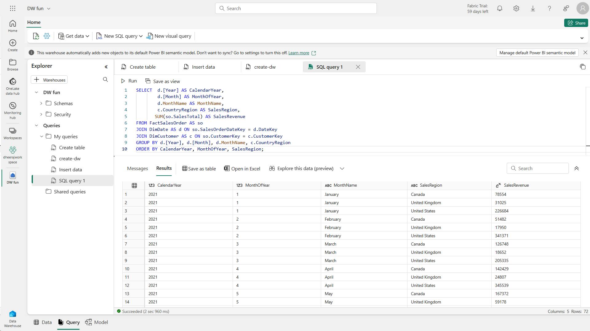
vi. Create a view
A data warehouse in Microsoft Fabric has many of the same capabilities you may be used to in relational databases.
For example, you can create database objects like views and stored procedures to encapsulate SQL logic.
IF EXISTS (
    SELECT * FROM sys.sysobjects
    WHERE name = 'vSalesByRegion')
DROP VIEW dbo.vSalesByRegion;
GO

CREATE VIEW vSalesByRegion
AS
SELECT  d.[Year] AS CalendarYear,
        d.[Month] AS MonthOfYear,
        d.MonthName AS MonthName,
        c.CountryRegion AS SalesRegion,
       SUM(so.SalesTotal) AS SalesRevenue
FROM FactSalesOrder AS so
JOIN DimDate AS d ON so.SalesOrderDateKey = d.DateKey
JOIN DimCustomer AS c ON so.CustomerKey = c.CustomerKey
GROUP BY d.[Year], d.[Month], d.MonthName, c.CountryRegion;
SELECT CalendarYear, MonthName, SalesRegion, SalesRevenue
FROM vSalesByRegion
ORDER BY CalendarYear, MonthOfYear, SalesRegion;
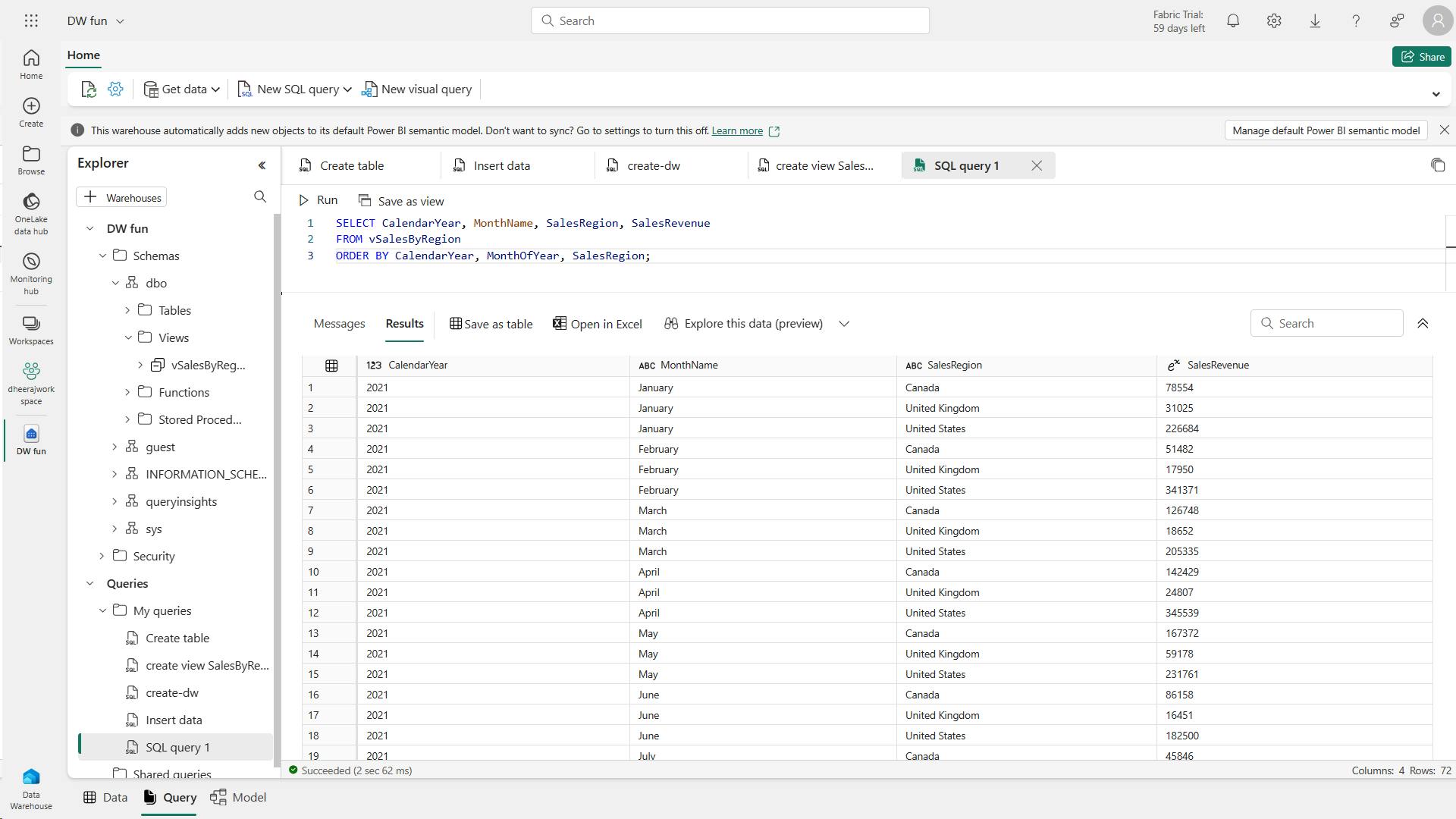
vii. Create a visual query
Instead of writing SQL code, you can use the graphical query designer to query the tables in your data warehouse.
This experience is similar to Power Query online, where you can create data transformation steps with no code.
For more complex tasks, you can use Power Query’s M (Mashup) language.
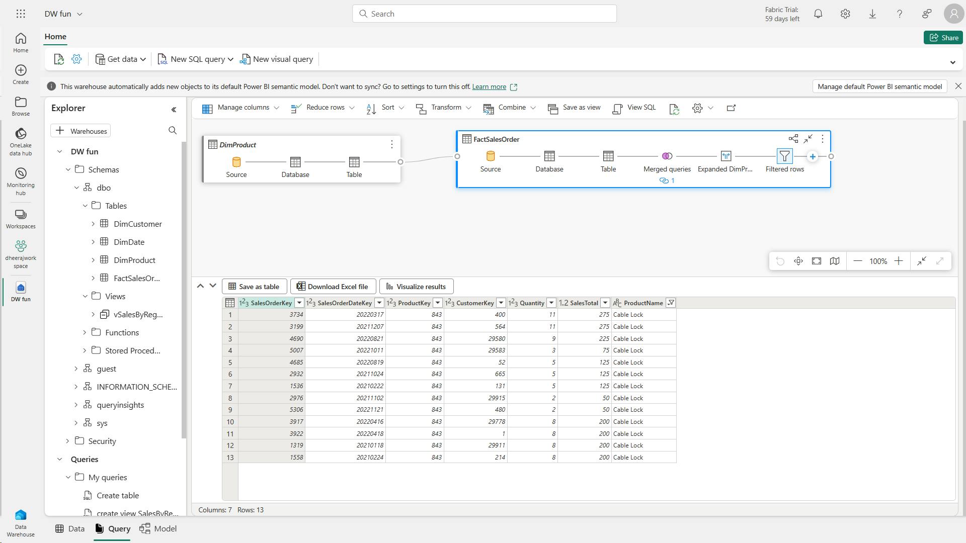
viii. Visualize your data
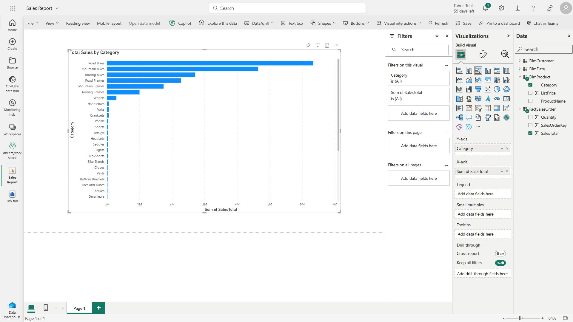
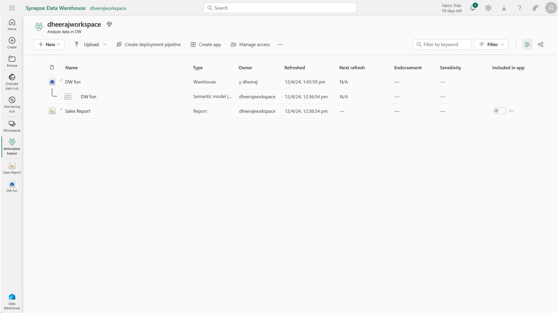
ix. Clean up resources
8. Knowledge check
Which type of table should an insurance company use to store supplier attribute details for aggregating claims?
A dimension table stores attributes used to group numeric measures.
What is a semantic model in the data warehouse experience?
A semantic model in the data warehouse experience provides a way to organize and structure data in a way that is meaningful to business users, enabling them to easily access and analyze data.
What is the purpose of item permissions in a workspace?
By granting access to a single data warehouse using item permissions, you can enable downstream consumption of data.
9. Summary
In this module, you learned about data warehouses and dimensional modeling, created a data warehouse, loaded, queried, and visualized data, and described semantic models and how they're used for downstream reporting.
data warehouses in Fabric, create a data warehouse, load, query, and visualize data.
Fabric's data warehouse provides full SQL semantics, including the ability to insert, update, and delete data in the tables.
fact tables(numerical data, large number of rows) and dimension tables(descriptive information, small number of rows, surrogate key, alternate key),
Star schema, snowflake schema,
data warehouse enables you to manipulate the data
data warehouse experience in Fabric, you can build a relational layer on top of physical data in the Lakehouse and expose it to analysis and reporting tools.
ingest data into data warehouse = Pipelines, Dataflows, cross-database querying, and the COPY INTO command
copy data from an external location into a table in the data warehouse using the COPY INTO syntax
SQL query loads data from a CSV file stored in Azure Blob Storage into a table called "Region" in the Fabric data warehouse.
staging tables - process of loading data into those tables, use T-SQL commands to load data from files into staging tables in the data warehouse,
Staging tables are temporary tables that can be used to perform data cleansing, data transformations, and data validation.
implement a data warehouse load process
query data in the lakehouse directly from the data warehouse using cross-database querying
create tables, views, and stored procedures to query data in the data warehouse and Lakehouse.
Visual query editor provides a no-code, drag-and-drop experience to create your queries
SQL query editor to write your queries.
A semantic model defines the relationships between the different tables in the semantic model, the rules for how data is aggregated and summarized, and the calculations or measures that are used to derive insights from the data.
semantic model defines - relationships/cardinality, rules for how data is aggregated and summarized, calculations or measures
Measures are the metrics that you want to analyze in your data warehouse.
Measures are calculated fields that are based on the data in the tables in your data warehouse using the Data Analysis Expressions (DAX) formula language.
sys.dm_exec_requests
a data warehouse provides a relational database for large-scale analytics. Unlike the default read-only SQL endpoint for tables defined in a lakehouse, a data warehouse provides full SQL semantics; including the ability to insert, update, and delete data in the tables.
A warehouse is a relational database in which you can define tables and other objects.
buildreport.
Learning objectives
In this module, you'll learn how to:
Describe data warehouses in Fabric
Understand a data warehouse vs a data Lakehouse
Work with data warehouses in Fabric
Create and manage fact tables and dimensions within a data warehouse
X. Load data into a Microsoft Fabric data warehouse
Data warehouse in Microsoft Fabric is a comprehensive platform for data and analytics, featuring advanced query processing and full transactional T-SQL capabilities for easy data management and analysis.
1. Introduction
Microsoft Fabric Data Warehouse is a complete platform for data, analytics, and AI (Artificial Intelligence).
It refers to the process of storing, organizing, and managing large volumes of structured and semi-structured data.
Microsoft Fabric Data Warehouse is a complete platform for data, analytics, and AI (Artificial Intelligence). It refers to the process of storing, organizing, and managing large volumes of structured and semi-structured data.
Data warehouse in Microsoft Fabric is powered up with Synapse Analytics by offering a rich set of features that make it easier to manage and analyze data. It includes advanced query processing capabilities, and supports the full transactional T-SQL capabilities like an enterprise data warehouse.
Unlike a dedicated SQL pool in Synapse Analytics, a warehouse in Microsoft Fabric is centered around a single data lake. The data in the Microsoft Fabric warehouse is stored in the Parquet file format. This setup allows users to focus on tasks such as data preparation, analysis, and reporting. It takes advantage of the SQL engine’s extensive capabilities, where a unique copy of their data is stored in Microsoft OneLake.
i. Understand the ETL (Extract, Transform and Load) process
ETL provides the foundation for data analytics and data warehouse workstreams.
Let's review some aspects of data manipulation in an ETL process.
| Description | |
| Data extraction | It involves connecting to the source system and collecting necessary data for analytical processing. |
| Data transformation | It involves a series of steps performed on the extracted data to convert it into a standard format. Combining data from different tables, cleaning data, deduplicating data and performing data validations. |
| Data loading | The extracted and transformed data are loaded into the fact and dimension tables. For an incremental load, this involves periodically applying ongoing changes as per requirement. This process often involves reformatting the data to ensure its quality and compatibility with the data warehouse schema. |
| Post-load optimizations | Once the data is loaded, certain optimizations can be performed to enhance the performance of the data warehouse. |
All these steps in the ETL process can run in parallel depending on the scenario. As soon as some data is ready, it's loaded without waiting for the previous steps to be completed.
In the next units, we'll explore various ways of loading data in a warehouse, and how they can facilitate the tasks of building a data warehouse workload.
2. Explore data load strategies
In Microsoft Fabric, there are many ways you can choose to load data in a warehouse.
This step is fundamental as it ensures that high-quality, transformed or processed data is integrated into a single repository.
Also, the efficiency of data loading directly impacts the timeliness and accuracy of analytics, making it vital for real-time decision-making processes.
Investing time and resources in designing and implementing a robust data loading strategy is essential for the success of the data warehouse project.
i. Understand data ingestion and data load operations
While both processes are part of the ETL (Extract, Transform, Load) pipeline in a data warehouse scenario, they usually serve different purposes.
Data ingestion/extract is about moving raw data from various sources into a central repository.
On the other hand, data loading involves taking the transformed or processed data and loading it into the final storage destination for analysis and reporting.
All Fabric data items like data warehouses and lakehouses store their data automatically in OneLake in Delta Parquet format.
ii. Stage your data
You may have to build and work with auxiliary objects involved in a load operation such as tables, stored procedures, and functions. These auxiliary objects are commonly referred to as staging. Staging objects act as temporary storage and transformation areas. They can share resources with a data warehouse, or live in its own storage area.
Staging serves as an abstraction layer, simplifying and facilitating the load operation to the final tables in the data warehouse.
Also, staging area provides a buffer that can help to minimize the impact of the load operation on the performance of the data warehouse. This is important in environments where the data warehouse needs to remain operational and responsive during the data loading process.
iii. Review type of data loads
There are two types of data loads to consider when loading a data warehouse.
| Load Type | Description | Operation | Duration | Complexity | Best used |
| Full (initial) load | The process of populating the data warehouse for the first time. | All the tables are truncated and reloaded, and the old data is lost | It may take longer to complete due to the amount of data being handled | Easier to implement as there's no history preserved | This method is typically used when setting up a new data warehouse, or when a complete refresh of the data is required |
| Incremental load | The process of updating the data warehouse with the changes since the last update | The history is preserved, and tables are updated with new information | Takes less time than the initial load | Implementation is more complex than the initial load | This method is commonly used for regular updates to the data warehouse, such as daily or hourly updates. It requires mechanisms to track changes in the source data since the last load. |
An ETL (Extract, Transform, Load) process for a data warehouse doesn't always need both the full load and the incremental load. In some cases, a combination of both methods might be used.
The choice between a full load and an incremental load depends on many factors such as the amount of data, the characteristics of the data, and the requirements of the data warehouse.
iv. Load a dimension table
Think of a dimension table as the "who, what, where, when, why” of your data warehouse.
It’s like the descriptive backdrop that gives context to the raw numbers found in the fact tables.
For example, if you’re running an online store, your fact table might contain the raw sales data - how many units of each product were sold. But without a dimension table, you wouldn’t know who bought those products, when they were bought, or where the buyer is located.
v. Slowly changing dimensions (SCD)
Slowly Changing Dimensions change over time, but at a slow pace and unpredictably. For example, a customer’s address in a retail business. When a customer moves, their address changes. If you overwrite the old address with the new one, you lose the history. But if you want to analyze historical sales data, you might need to know where the customer lived at the time of each sale. This is where SCDs come into play.
There are several types of slowly changing dimensions in a data warehouse, with type 1 and type 2 being the most frequently used.
Type 0 SCD: The dimension attributes never change.
Type 1 SCD: Overwrites existing data, doesn't keep history.
Type 2 SCD: Adds new records for changes, keeps full history for a given natural key.
Type 3 SCD: History is added as a new column.
Type 4 SCD: A new dimension is added.
Type 5 SCD: When certain attributes of a large dimension change over time, but using type 2 isn't feasible due to the dimension’s large size.
Type 6 SCD: Combination of type 2 and type 3.
In type 2 SCD, when a new version of the same element is brought to the data warehouse, the old version is considered expired and the new one becomes active.
The following example shows how to handle changes in a type 2 SCD for the Dim_Products table using T-SQL.
IF EXISTS (SELECT 1 FROM Dim_Products WHERE SourceKey = @ProductID AND IsActive = 'True')
BEGIN
    -- Existing product record
    UPDATE Dim_Products
    SET ValidTo = GETDATE(), IsActive = 'False'
    WHERE SourceKey = @ProductID AND IsActive = 'True';
END
ELSE
BEGIN
    -- New product record
    INSERT INTO Dim_Products (SourceKey, ProductName, StartDate, EndDate, IsActive)
    VALUES (@ProductID, @ProductName, GETDATE(), '9999-12-31', 'True');
END
The mechanism for detecting changes in source systems is crucial for determining when records are inserted, updated, or deleted.
Change Data Capture (CDC), change tracking,and triggers are all features available for managing data tracking in source systems such as SQL Server.
vi. Load a fact table
Let's consider an example where we load a Fact_Sales table in a data warehouse. This table contains sales transactions data with columns such as FactKey, DateKey, ProductKey, OrderID, Quantity, Price, and LoadTime.
Assume we have a source table Order_Detail in an OLTP system with columns: OrderID, OrderDate, ProductID, Quantity, and Price.
The following T-SQL script example load the Fact_Sales table.
-- Lookup keys in dimension tables
INSERT INTO Fact_Sales (DateKey, ProductKey, OrderID, Quantity, Price, LoadTime)
SELECT d.DateKey, p.ProductKey, o.OrderID, o.Quantity, o.Price, GETDATE()
FROM Order_Detail o
JOIN Dim_Date d ON o.OrderDate = d.Date
JOIN Dim_Product p ON o.ProductID = p.ProductID;
3. Use data pipelines to load a warehouse
Microsoft Fabric’s Warehouse provides integrated data ingestion tools, enabling users to load and ingest data into warehouses on a large scale through either coding or noncoding experiences.
Data pipeline is the cloud-based service for data integration, which enables the creation of workflows for data movement and data transformation at scale.
You can create and schedule data pipelines that can ingest and load data from disparate data stores.
You can build complex ETL, or ELT processes that transform data visually with data flows.
Most of the functionality of data pipelines in Microsoft Fabric comes from Azure Data Factory, allowing for seamless integration and utilization of its features within the Microsoft Fabric ecosystem.
i. Create a data pipeline
From the workspace: Select + New, then select Data pipeline. If it's not visible in the list, select More options, then find Data pipeline under the Data Factory section.
From the warehouse asset - Select Get Data, and then New data pipeline.
There are three options available when creating a pipeline.
| Option | Description |
| 1. Add pipeline activity | Launches the pipeline editor where you can create your own pipeline. |
| 2. Copy data | Launches an assistant to copy data from various data sources to a data destination. A new pipeline activity is generated at the end with a preconfigured Copy Data task. |
| 3. Choose a task to start | You can choose from a collection of predefined templates to assist you in initiating pipelines based on many scenarios. |
ii. Configure the copy data assistant
The copy data assistant provides a step-by-step interface that facilitates the configuration of a Copy Data task.
Choose data source: Select a connector, and provide the connection information.
Connect to a data source: Select, preview, and choose the data. This can be done from tables or views, or you can customize your selection by providing your own query.
Choose data destination: Select the data store as the destination.
Connect to data destination: Select and map columns from source to destination. You can load to a new or existing table.
Settings: Configure other settings like staging, and default values.
After you copy the data, you can use other tasks to further transform and analyze it. You can also use the Copy Data task to publish transformation and analysis results for business intelligence (BI) and application consumption.
iii. Schedule a data pipeline
You can schedule your data pipeline by selecting Schedule from the data pipeline editor.
We recommend data pipelines for a code-free or low-code experience due to the graphical user interface. They're ideal for data workflows that run at a schedule, or that connects to different data sources.
4. Load data using T-SQL
SQL developers or citizen developers, who are often well-versed in the SQL engine and adept at using T-SQL, will find the Warehouse in Microsoft Fabric favorable.
This is because the Warehouse is powered by the same SQL engine they're familiar with, enabling them to perform complex queries and data manipulations.
These operations include filtering, sorting, aggregating, and joining data from different tables.
The SQL engine’s wide range of functions and operators further allows for sophisticated data analysis and transformations at the database level.
i. Use COPY statement
The COPY statement serves as the main method for importing data into the Warehouse. It facilitates efficient data ingestion from an external Azure storage account.
It offers flexibility, allowing you to specify the format of the source file, designate a location for storing rows that are rejected during the import process, skip header rows, among other configurable options.
The option to store rejected rows separately is useful for data cleaning and quality control. It allows you to easily identify and investigate any issues with the data that weren't successfully imported.
To connect to an Azure storage account, you need to use either Shared Access Signature (SAS) or Storage Account Key (SAK).
Note:
The COPY statement currently supports the PARQUET and CSV file formats.
ii. Handle error
The option to use a different storage account for the ERRORFILE location (REJECTED_ROW_LOCATION) allows for better error handling and debugging.
It makes it easier to isolate and investigate any issues that occur during the data loading process. ERRORFILE only applies to CSV.
iii. Load multiple files
The ability to specify wildcards and multiple files in the storage location path allows the COPY statement to handle bulk data loading efficiently.
This is useful when dealing with large datasets distributed across multiple files.
Multiple file locations can only be specified from the same storage account and container via a comma-separated list.
COPY my_table
FROM 'https://myaccount.blob.core.windows.net/myblobcontainer/folder0/*.csv,
    https://myaccount.blob.core.windows.net/myblobcontainer/folder1/'
WITH (
    FILE_TYPE = 'CSV',
    CREDENTIAL=(IDENTITY= 'Shared Access Signature', SECRET='<Your_SAS_Token>')
    FIELDTERMINATOR = '|'
)
The following example shows how to load a PARQUET file.
COPY INTO test_parquet
FROM 'https://myaccount.blob.core.windows.net/myblobcontainer/folder1/*.parquet'
WITH (
    CREDENTIAL=(IDENTITY= 'Shared Access Signature', SECRET='<Your_SAS_Token>')
)
Ensure that all the files have the same structure (that is, same columns in the same order) and that this structure matches the structure of the target table.
iv. Load table from other warehouses and lakehouses
You can load data from various data assets in a workspace, such as other warehouses and lakehouses.
To reference the data asset, ensure that you use three-part naming to combine data from tables on these workspace assets.
You can then use CREATE TABLE AS SELECT (CTAS) and INSERT...SELECT to load the data into the warehouse.
| SQL Statement | Description |
CREATE TABLE AS SELECT | Allows you to create a new table based on the output of a SELECT statement. This operation is often used for creating a copy of a table or for transforming and loading the results of complex queries. |
INSERT...SELECT | Allows you to insert data from one table into another. It’s useful when you want to copy data from one table to another without creating a new table. |
In a scenario where an analyst needs data from both a warehouse and a lakehouse, they can use this feature to combine the data. They can then load this combined data into the warehouse for analysis. This feature is useful when data is distributed across many assets in a workspace.
he following query creates a new table in the analysis_warehouse that combines data from the sales_warehouse and the social_lakehouse using the product_id as the common key. The new table can then be used for further analysis.
CREATE TABLE [analysis_warehouse].[dbo].[combined_data]
AS
SELECT
FROM [sales_warehouse].[dbo].[sales_data] sales
INNER JOIN [social_lakehouse].[dbo].[social_data] social
ON sales.[product_id] = social.[product_id];
All the Warehouses that share the same workspace are integrated into the same logical SQL server. If you use SQL client tools such as SQL Server Management Studio, you can easily perform a cross-database query like in any SQL Server instance.
MyWarehouse and Sales are both warehouse assets that share the same workspace.
If you’re using the object Explorer from the workspace to query your Warehouses, you need to add them explicitly. The warehouses added will also be visible from the Visual query editor.
When using T-SQL, data can be efficiently loaded into a warehouse in Microsoft Fabric through the COPY statement, or from other warehouses and lakehouses within the same workspace, allowing for seamless data management and analysis.
5. Load and transform data with Dataflow Gen2
Dataflow Gen2 is the new generation of dataflows. It provides a comprehensive Power Query experience, guiding you through each step of importing data into your dataflow. The process of creating dataflows has been simplified, reducing the number of steps involved.
You can use dataflows in data pipelines to ingest data into a lakehouse or warehouse, or to define a dataset for a Power BI report.
i. Create a dataflow
ii. Import data
iii. Transform data with Copilot
iv. Add a data destination
With the Add data destination feature, you can separate your ETL logic and destination storage. This separation can lead to cleaner, more maintainable code and can make it easier to modify either the ETL process or the storage configuration without affecting the other.
Once the data is transformed, the next step is to add a destination step. On the Query settings tab, select + to add a destination step in your dataflow.
v. Publish a dataflow
Publishing makes your transformations and data loading operations live, allowing the dataflow to be executed either manually or on a schedule. This process encapsulates your ETL operations into a single and reusable unit, streamlining your data management workflow.
Any changes made in the dataflow take effect when it’s published. So, always ensure to publish your dataflow after making any relevant modifications.
6. Exercise: Load data into a warehouse in Microsoft Fabric
In Microsoft Fabric, a data warehouse provides a relational database for large-scale analytics.
Unlike the default read-only SQL endpoint for tables defined in a lakehouse, a data warehouse provides full SQL semantics; including the ability to insert, update, and delete data in the tables.
i. Create a workspace
ii. Create a lakehouse and upload files
In our scenario, since we don’t have any available data, we must ingest data to be used for loading the warehouse.
You’ll create a data lakehouse for the data files you’re going to use to load the warehouse.
Download the file for this exercise from https://github.com/MicrosoftLearning/dp-data/raw/main/sales.csv
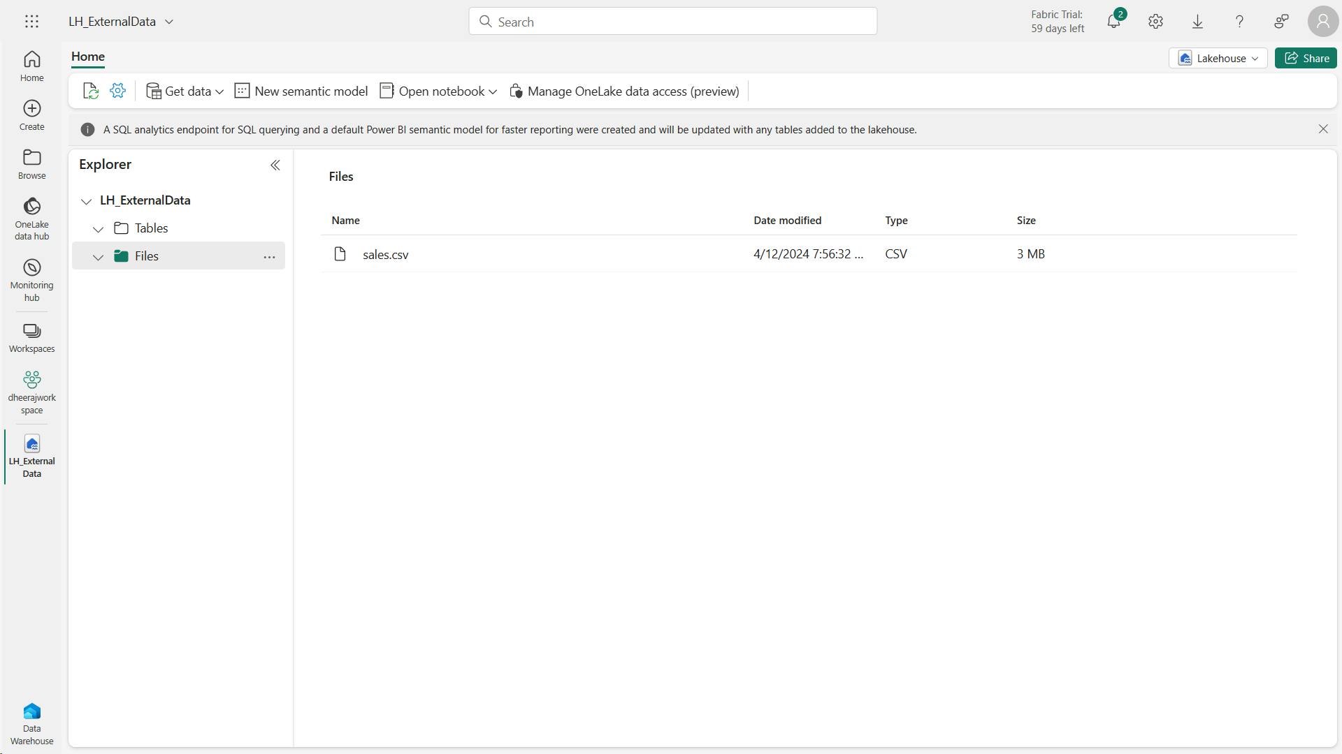
iii. Create a table in the lakehouse
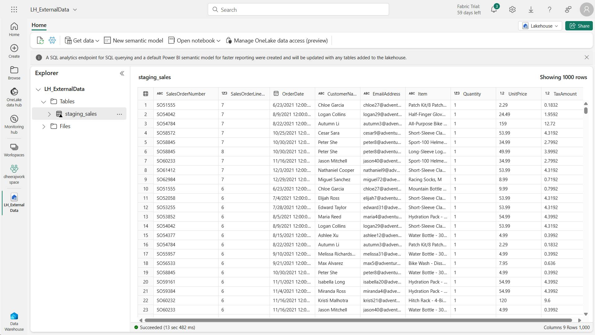
iv. Create a warehouse
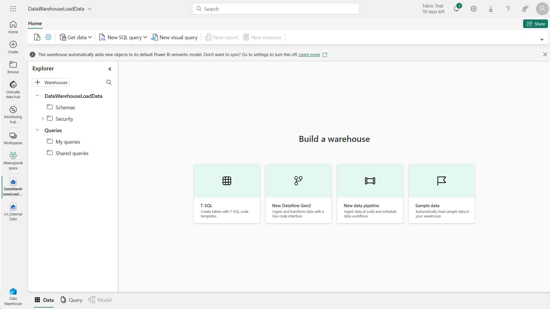
v. Create fact table, dimensions and view
Let’s create the fact tables and dimensions for the Sales data. You’ll also create a view pointing to a lakehouse, this simplifies the code in the stored procedure we’ll use to load.
IF EXISTS (SELECT * FROM sys.schemas WHERE name ='Sales')
 DROP SCHEMA [Sales]
GO

CREATE SCHEMA [Sales]
GO

IF NOT EXISTS (SELECT * FROM sys.tables WHERE name='Fact_Sales' AND SCHEMA_NAME(schema_id)='Sales')
CREATE TABLE Sales.Fact_Sales (
    CustomerID VARCHAR(255) NOT NULL,
    ItemID VARCHAR(255) NOT NULL,
    SalesOrderNumber VARCHAR(30),
    SalesOrderLineNumber INT,
    OrderDate DATE,
    Quantity INT,
    TaxAmount FLOAT,
    UnitPrice FLOAT
);

IF NOT EXISTS (SELECT * FROM sys.tables WHERE name='Dim_Customer' AND SCHEMA_NAME(schema_id)='Sales')
    CREATE TABLE Sales.Dim_Customer (
        CustomerID VARCHAR(255) NOT NULL,
        CustomerName VARCHAR(255) NOT NULL,
        EmailAddress VARCHAR(255) NOT NULL
    );

ALTER TABLE Sales.Dim_Customer add CONSTRAINT PK_Dim_Customer PRIMARY KEY NONCLUSTERED (CustomerID) NOT ENFORCED
GO

IF NOT EXISTS (SELECT * FROM sys.tables WHERE name='Dim_Item' AND SCHEMA_NAME(schema_id)='Sales')
    CREATE TABLE Sales.Dim_Item (
        ItemID VARCHAR(255) NOT NULL,
        ItemName VARCHAR(255) NOT NULL
    );

ALTER TABLE Sales.Dim_Item add CONSTRAINT PK_Dim_Item PRIMARY KEY NONCLUSTERED (ItemID) NOT ENFORCED
GO
Note:
In a data warehouse, foreign key constraints are not always necessary at the table level.
While foreign key constraints can help ensure data integrity, they can also add overhead to the ETL (Extract, Transform, Load) process and slow down data loading.
The decision to use foreign key constraints in a data warehouse should be based on a careful consideration of the trade-offs between data integrity and performance.
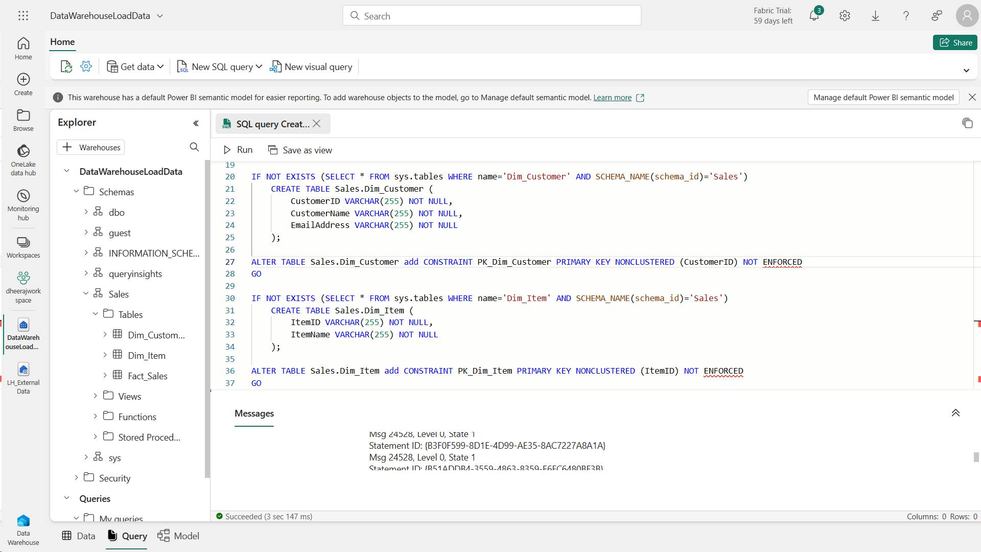
CREATE VIEW Sales.Staging_Sales
AS
SELECT * FROM [<your lakehouse name>].[dbo].[staging_sales];
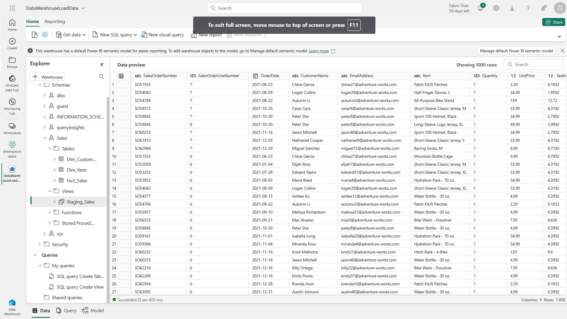
vi. Load data to the warehouse
Now that the fact and dimensions tables are created, let’s create a stored procedure to load the data from our lakehouse into the warehouse.
Because of the automatic SQL endpoint created when we create the lakehouse, you can directly access the data in your lakehouse from the warehouse using T-SQL and cross-database queries.
CREATE OR ALTER PROCEDURE Sales.LoadDataFromStaging (@OrderYear INT)
AS
BEGIN
-- Load data into the Customer dimension table
    INSERT INTO Sales.Dim_Customer (CustomerID, CustomerName, EmailAddress)
    SELECT DISTINCT CustomerName, CustomerName, EmailAddress
    FROM [Sales].[Staging_Sales]
    WHERE YEAR(OrderDate) = @OrderYear
    AND NOT EXISTS (
        SELECT 1
        FROM Sales.Dim_Customer
        WHERE Sales.Dim_Customer.CustomerName = Sales.Staging_Sales.CustomerName
        AND Sales.Dim_Customer.EmailAddress = Sales.Staging_Sales.EmailAddress
    );

    -- Load data into the Item dimension table
    INSERT INTO Sales.Dim_Item (ItemID, ItemName)
    SELECT DISTINCT Item, Item
    FROM [Sales].[Staging_Sales]
    WHERE YEAR(OrderDate) = @OrderYear
    AND NOT EXISTS (
        SELECT 1
        FROM Sales.Dim_Item
        WHERE Sales.Dim_Item.ItemName = Sales.Staging_Sales.Item
    );

    -- Load data into the Sales fact table
    INSERT INTO Sales.Fact_Sales (CustomerID, ItemID, SalesOrderNumber, SalesOrderLineNumber, OrderDate, Quantity, TaxAmount, UnitPrice)
    SELECT CustomerName, Item, SalesOrderNumber, CAST(SalesOrderLineNumber AS INT), CAST(OrderDate AS DATE), CAST(Quantity AS INT), CAST(TaxAmount AS FLOAT), CAST(UnitPrice AS FLOAT)
    FROM [Sales].[Staging_Sales]
    WHERE YEAR(OrderDate) = @OrderYear;
END
EXEC Sales.LoadDataFromStaging 2021
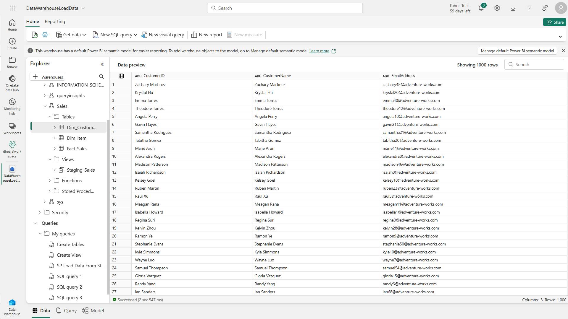
vii. Run analytical queries
This query shows the customers by total sales for the year of 2021. The customer with the highest total sales for the specified year is Jordan Turner, with total sales of 14686.69.
 SELECT c.CustomerName, SUM(s.UnitPrice * s.Quantity) AS TotalSales
 FROM Sales.Fact_Sales s
 JOIN Sales.Dim_Customer c
 ON s.CustomerID = c.CustomerID
 WHERE YEAR(s.OrderDate) = 2021
 GROUP BY c.CustomerName
 ORDER BY TotalSales DESC;
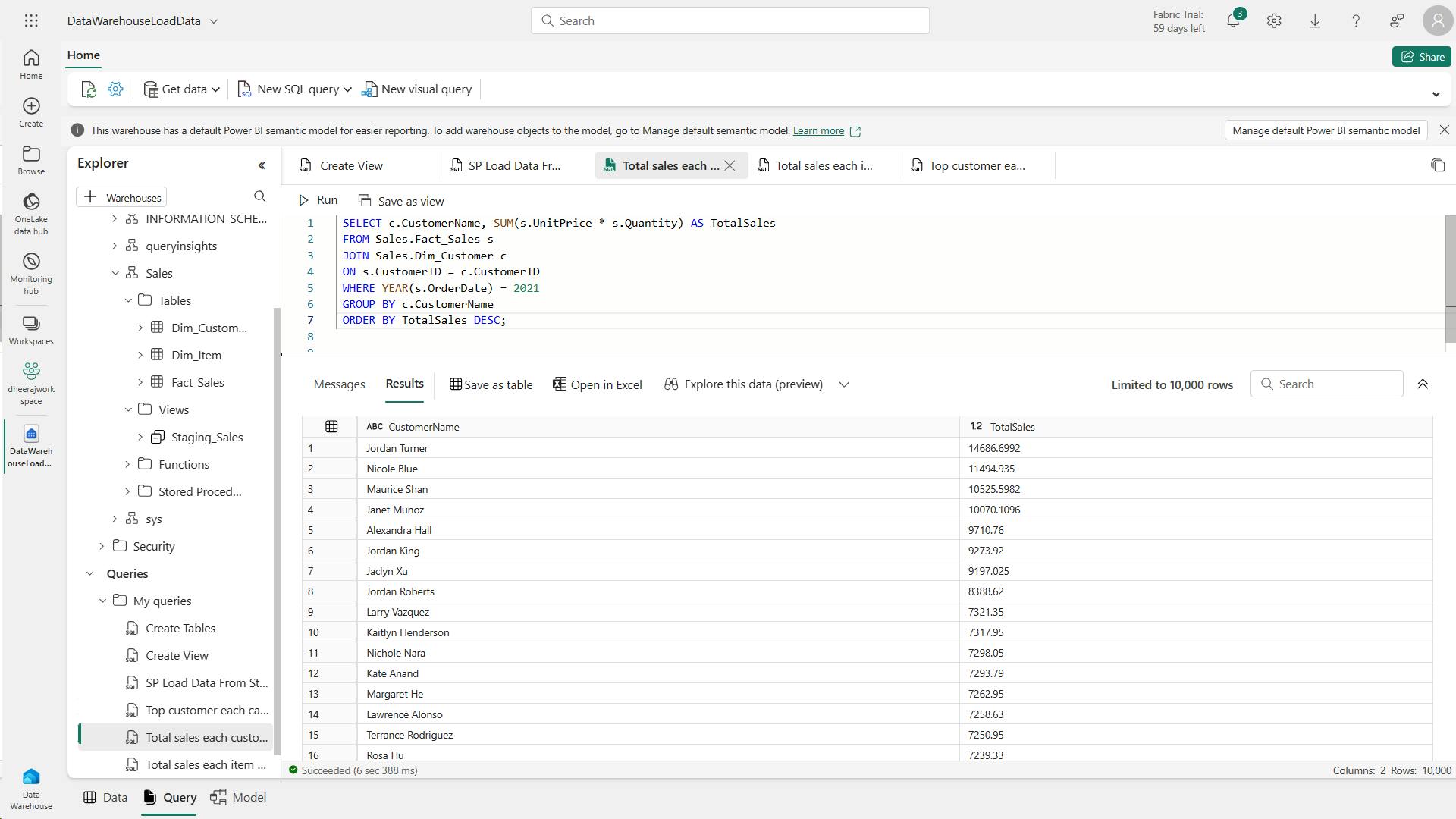
This query shows the top-selling items by total sales for the year of 2021.
These results suggest that the Mountain-200 bike model, in both black and silver colors, was the most popular item among customers in 2021.
 SELECT i.ItemName, SUM(s.UnitPrice * s.Quantity) AS TotalSales
 FROM Sales.Fact_Sales s
 JOIN Sales.Dim_Item i
 ON s.ItemID = i.ItemID
 WHERE YEAR(s.OrderDate) = 2021
 GROUP BY i.ItemName
 ORDER BY TotalSales DESC;
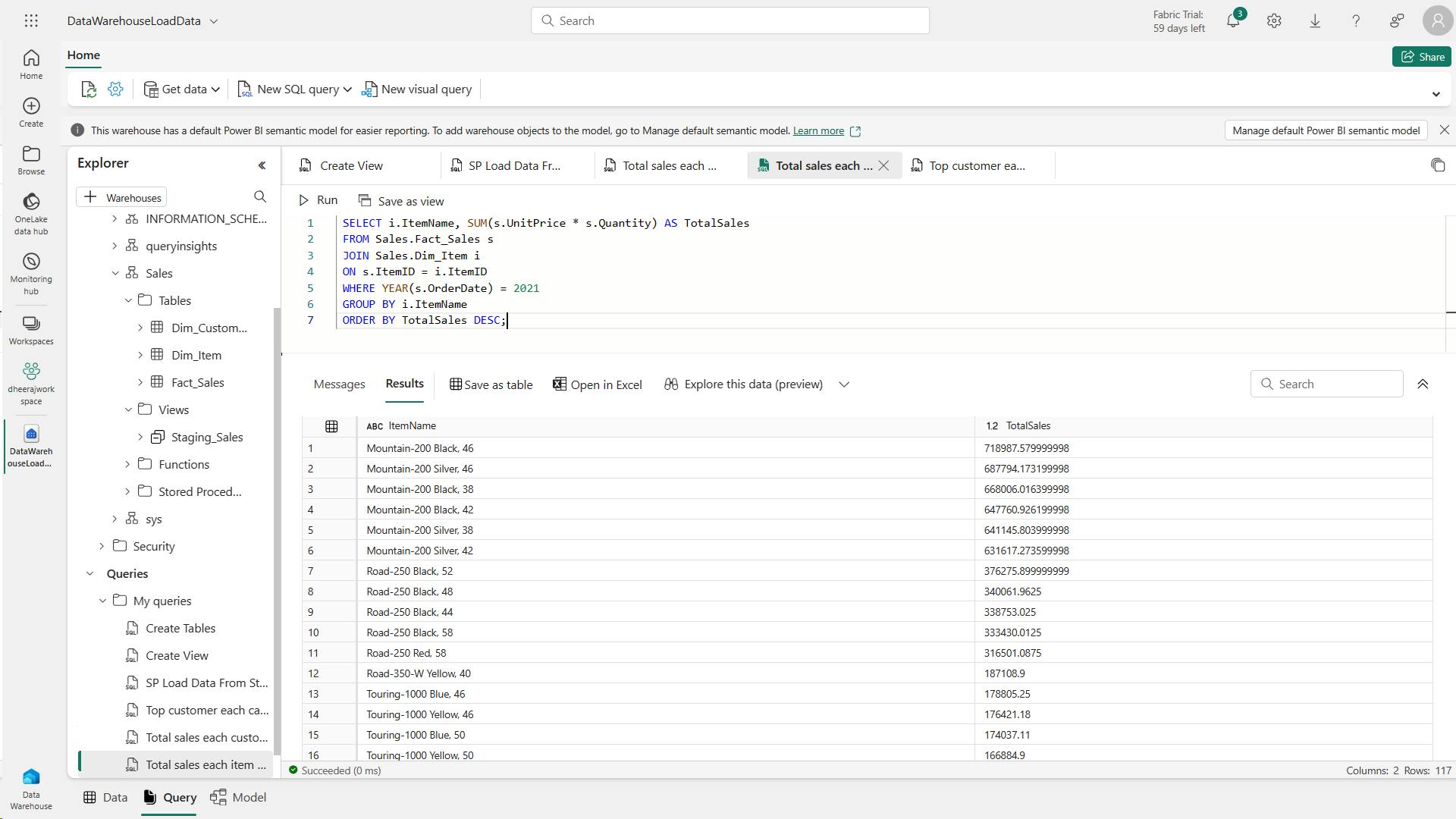
The results of this query show the top customer for each of the categories: Bike, Helmet, and Gloves, based on their total sales. For example, Joan Coleman is the top customer for the Gloves category
WITH CategorizedSales AS (
SELECT
    CASE
        WHEN i.ItemName LIKE '%Helmet%' THEN 'Helmet'
        WHEN i.ItemName LIKE '%Bike%' THEN 'Bike'
        WHEN i.ItemName LIKE '%Gloves%' THEN 'Gloves'
        ELSE 'Other'
    END AS Category,
    c.CustomerName,
    s.UnitPrice * s.Quantity AS Sales
FROM Sales.Fact_Sales s
JOIN Sales.Dim_Customer c
ON s.CustomerID = c.CustomerID
JOIN Sales.Dim_Item i
ON s.ItemID = i.ItemID
WHERE YEAR(s.OrderDate) = 2021
),
RankedSales AS (
    SELECT
        Category,
        CustomerName,
        SUM(Sales) AS TotalSales,
        ROW_NUMBER() OVER (PARTITION BY Category ORDER BY SUM(Sales) DESC) AS SalesRank
    FROM CategorizedSales
    WHERE Category IN ('Helmet', 'Bike', 'Gloves')
    GROUP BY Category, CustomerName
)
SELECT Category, CustomerName, TotalSales
FROM RankedSales
WHERE SalesRank = 1
ORDER BY TotalSales DESC;
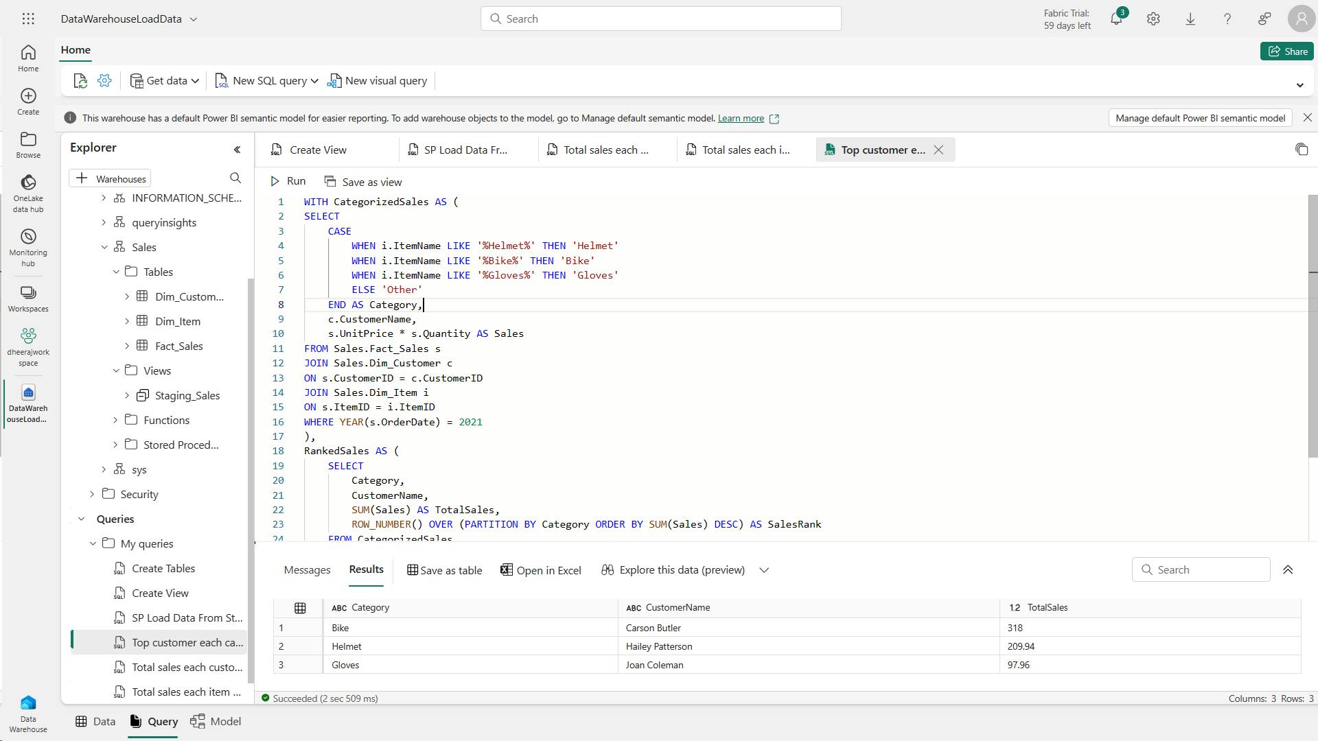
viii. Clean up resources
7. Knowledge check
What are the four data ingestion options available in Microsoft Fabric for loading data into a data warehouse?
COPY (Transact-SQL) statement, data pipelines, dataflows, and cross-warehouse.
COPY (Transact-SQL) statement, data pipelines, dataflows, and cross-warehouse are the four data ingestion options available in Microsoft Fabric for loading data into a data warehouse.
What are the supported data sources and file formats for the COPY (Transact-SQL) statement in Warehouse?
Azure Data Lake Storage (ADLS) Gen2 and Azure Blob Storage, with PARQUET and CSV file formats.
The COPY (Transact-SQL) statement currently supports the PARQUET and CSV file formats, and Azure Data Lake Storage (ADLS) Gen2 and Azure Blob Storage as data sources.
What is the recommended minimum file size when working with external data on files in Microsoft Fabric?
At least 4 MB.
When working with external data on files, we recommend that files are at least 4 MB in size.
8. Summary
There’s no one-size-fits-all solution for loading your data. The best approach depends on the specifics of your business requirement and the question you’re trying to answer.
When it comes to loading data in a data warehouse, there are several considerations to keep in mind.
| Description | |
| Load volume & frequency | Assess data volume and load frequency to optimize performance. |
| Governance | Any data that lands in OneLake is governed by default. |
| Data mapping | Manage mapping from source to staging to warehouse. |
| Dependencies | Understand dependencies in the data model for loading dimensions. |
| Script design | Design efficient import scripts considering column names, filtering rules, value mapping, and database indexing. |
Think of a dimension table as the "who, what, where, when, why” of your data warehouse.
It’s like the descriptive backdrop that gives context to the raw numbers found in the fact tables.
type 1 and type 2 the most frequently used slowly changing dimensions in a data warehouse
Load a Fact_Sales table in a data warehouse using INSERT INTO
All data in a Warehouse is automatically stored in the Delta Parquet format in OneLake.
data pipelines to load a warehouse
The COPY statement currently supports the PARQUET and CSV file formats.
Load data using T-SQL
COPY statement to handle bulk data loading efficiently.
Load table from other warehouses and lakehouses - CREATE TABLE AS SELECT (CTAS) and INSERT...SELECT
Learning objectives
In this module, you'll:
Learn different strategies to load data into a data warehouse in Microsoft Fabric.
Learn how to build a data pipeline to load a warehouse in Microsoft Fabric.
Learn how to load data in a warehouse using T-SQL, exercise.
Learn how to load and transform data with dataflow (Gen 2).
XI. Use tools to optimize Power BI performance
Use tools to develop, manage, and optimize Power BI data model and DAX query performance.
1. Introduction
You've built Power BI reports and they're running slow.
How do you identify the source of the problem?
The report could be slow because of
issues at the source,
the structure of the data model,
the visuals on the report page, or the environment.
In this module you'll learn how to use tools to optimize a data model, and which tools are useful in which scenarios.
2. Use Performance analyzer
Performance analyzer helps you understand how report elements like visuals and DAX queries are performing, helps you optimize at two of the four architecture levels, the data model and report visuals. EndFragment
i. Understand performance using Performance analyzer
The Performance Analyzer captures operations that occur in several major subsystems involved in executing a Power BI Report:
Operations that occur in several major subsystems:
a. Report Canvas
Report Canvas provides the user interface for Power BI reports including hosting visuals and filters, managing user interactions for consuming and authoring reports, and retrieving data for display.
The Report Canvas is written using web technologies and runs in web browsers or web browser components. The Report Canvas retrieves data using a high-level, internal, Power BI query language known as Semantic Query.
b. Data Shape Engine (DSE)
Data Shape Engine (DSE) evaluates Semantic Queries by generating and running one, or more DAX queries against a data model hosted inside Power BI, Power BI Desktop, Azure Analysis Services, or SQL Server Analysis Services.
c. Data Model Engine (AS)
Data Model Engine (AS) stores the data model and provides services to reports, such as DAX query evaluation.
The model may be hosted in Power BI, Power BI Desktop, Azure Analysis Services, or SQL Server Analysis Services.
Depending on the data model host, a model may be tabular or multidimensional.
Tabular models may contain in-memory tables, Direct Query tables, or a mix of such tables.
DAX queries against tables in Direct Query mode will trigger queries to the Direct Query data source.
For example, a DAX query against a Direct Query table backed by a SQL Server database will trigger one, or more, SQL queries.
ii. Use Performance analyzer
As users interact with visuals in Power BI reports, DAX queries are submitted to the dataset and cached into memory.
Because of this, you may need to clear the DAX query cache to get accurate results in the Performance analyzer.
You can clear the cache by either closing and re-opening your report, or using DAX Studio.
iii. Evaluate performance data further
For DAX queries with long duration times, means
it's likely that a measure is written poorly or
an issue has occurred with the data model.
The issue might be caused by the relationships, columns, or metadata in your model,
or it could be the status of the Auto date/time option.
3. Troubleshoot DAX performance by using DAX Studio
i. Understand the VertiPaq engine
By using compression algorithms and a multi-threaded query processor, the Analysis Services VertiPaq engine delivers fast access to tabular model objects and data by Power BI.
Power BI reads the content of your data source and transforms it in the internal VertiPaq columnar data structure, where each column is encoded and compressed. Dictionaries and indexes are created for each column.
Finally, data structures are created for relationships and computation and compression of calculated columns occurs.
DAX queries are being processed by two engines, the formula engine and the storage engine.
ii. Describe DAX Studio
iii. Optimize the data model
a. Optimize DAX queries
iv. View model metrics using VertiPaq Analyzer
VertiPaq Analyzer reports the memory consumption of the data model and can be used to quickly identify where you're spending the most memory.
The VertiPaq engine only stores data in memory in import models. If you're using DirectQuery, the VertiPaq engine simply sends that query to the source. This means that viewing the VertiPaq Analyzer Metrics will only be helpful for import or composite models.
Using the VertiPaq Analyzer in DAX Studio can help you easily identify and eliminate columns with high cardinality (including auto Date/time and floating-point decimal data types), and identify and remove columns that aren't used for anything.
4. Optimize a data model by using Best Practice Analyzer
The Best Practice Analyzer (BPA) in Tabular Editor can be used during the development of tabular models in Power BI or Analysis Services models.
i. Describe Tabular Editor
using Tabular Editor to run the BPA to ensure you're implementing data modeling best practices as you build.
ii. Describe the Best Practice Analyzer (BPA)
BPA is a set of rules run in Tabular Editor that notify you of potential modeling missteps or changes that you can make to improve your model design and performance. It includes recommendations for naming, user experience, and common optimizations that you can apply to improve performance.
iii. Run BPA in Tabular Editor
iv. Customize BPA for your organization
v. Incorporate the use of BPA into your Continuous Integration/Continuous Deployment (CI/CD) process
5. Exercise: Use tools to optimize Power BI performance
Exercise HTML page [Link]
https://microsoftlearning.github.io/mslearn-fabric/Instructions/Labs/16-use-tools-to-optimize-power-bi-performance.html
In this lab, you will learn how to use two external tools to help you develop, manage, and optimize data models and DAX queries.
In this lab, you learn how to:
Use Best Practice Analyzer (BPA).
Use DAX Studio.
Lab Files: [Link]
https://github.com/MicrosoftLearning/mslearn-fabric/tree/main/Allfiles/Labs/16
i. Use Best Practice Analyzer
In this exercise, you will install Tabular Editor 2 and load Best Practice Analyzer (BPA) rules. You will review the BPA rules, and then address specific issues found in the data model.
a. Download and Install Tabular Editor 2
Download and install Tabular Editor 2 to enable the creation of calculation groups. [Link]
b. Set up Power BI Desktop
Download the Sales Analysis starter file from https://aka.ms/fabric-optimize-starter
c. Review the data model
you will review the data model.
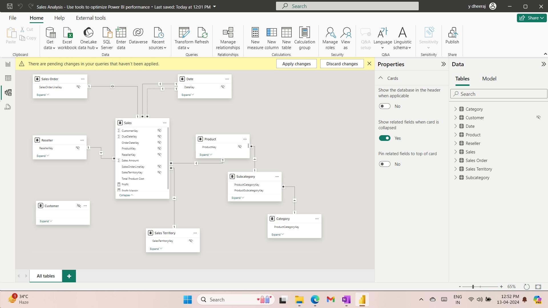
use BPA to detect model issues and fix them.
d. Load BPA rules
you will load BPA rules.
 System.Net.WebClient w = new System.Net.WebClient();

 string path = System.Environment.GetFolderPath(System.Environment.SpecialFolder.LocalApplicationData);
 string url = "https://raw.githubusercontent.com/microsoft/Analysis-Services/master/BestPracticeRules/BPARules.json";
 string downloadLoc = path+@"\TabularEditor\BPARules.json";
 w.DownloadFile(url, downloadLoc);
e. Review the BPA rules
you will review the BPA rules that you loaded in the previous task.
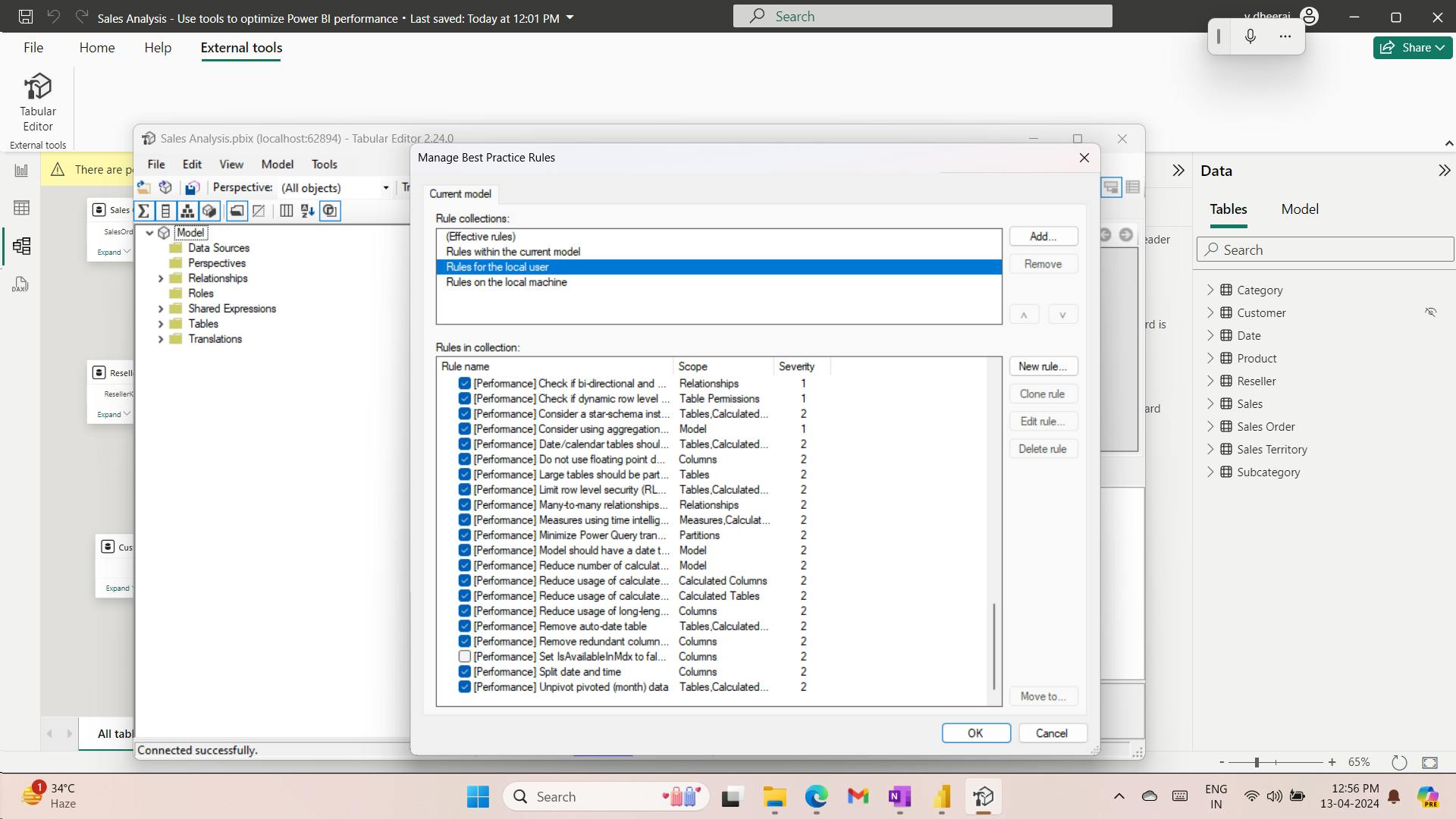
f. Address BPA issues
you will open BPA and review the results of the checks.
ii. Use DAX Studio
you’ll use DAX Studio to optimize DAX queries in the Power BI report file.
a. Download DAX Studio
[Link]
b. Use DAX studio to optimize a query
you will optimize a query by using an improved measure formula.
Download the Monthly Profit Growth.dax files from https://aka.ms/fabric-optimize-dax
The query defines two measures that determine monthly profit growth. Currently, the query only uses the first measure (at line 72). When a measure isn’t used, it doesn’t impact on the query execution.
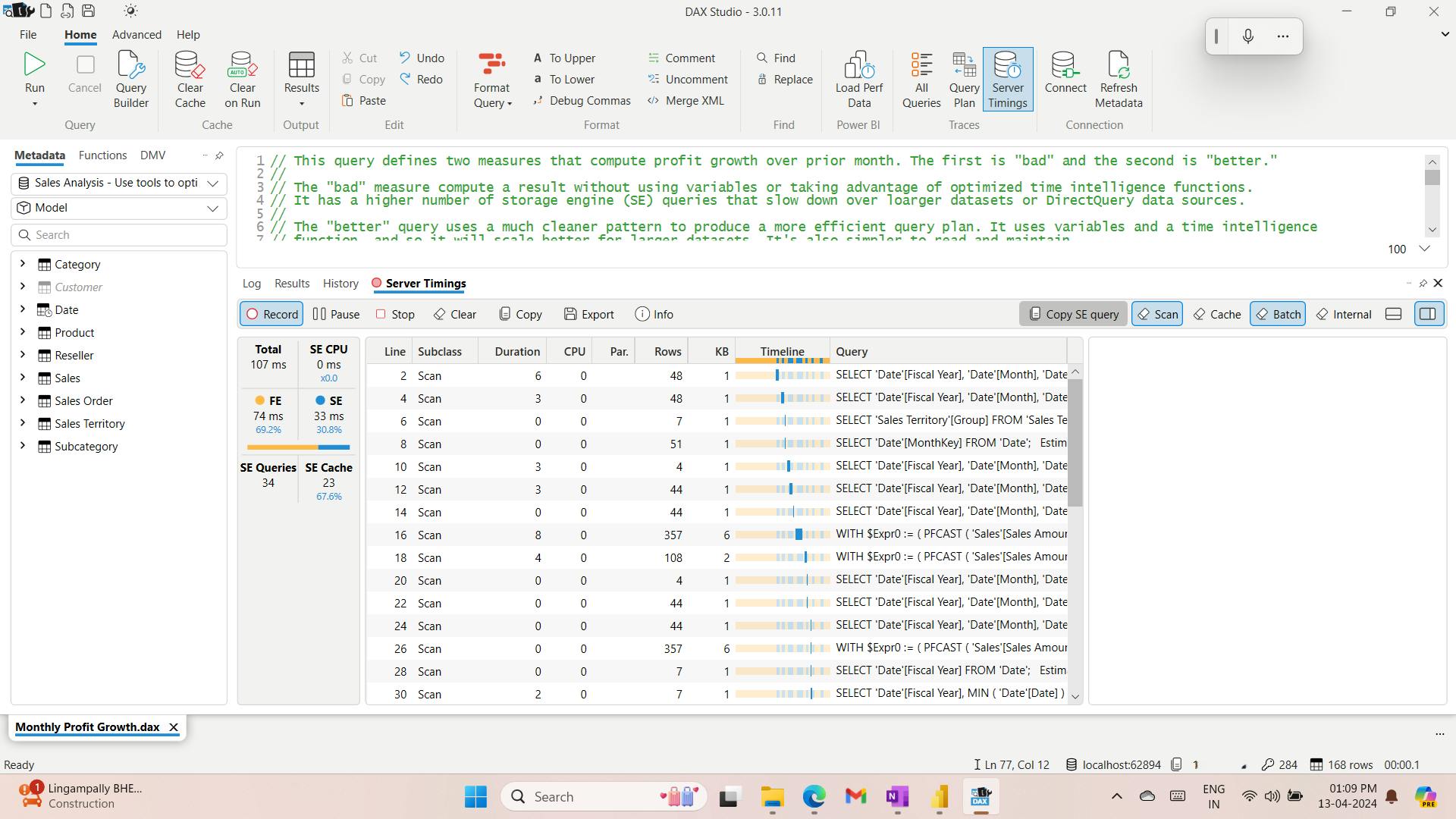
From top left to bottom right, the statistics tell you how many milliseconds it took to run the query, and the duration the storage engine (SE) CPU took. In this case (your results will differ), the formula engine (FE) took 69.2% of the time, while the SE took the remaining 30.8% of the time. There were 34 individual SE queries and 23 cache hits.
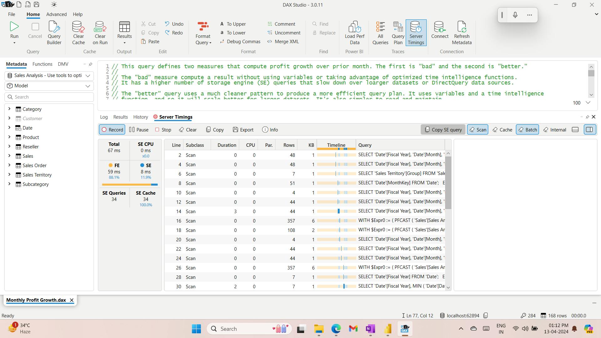
The second measure definition provides a more efficient result. You will now update the query to use the second measure.
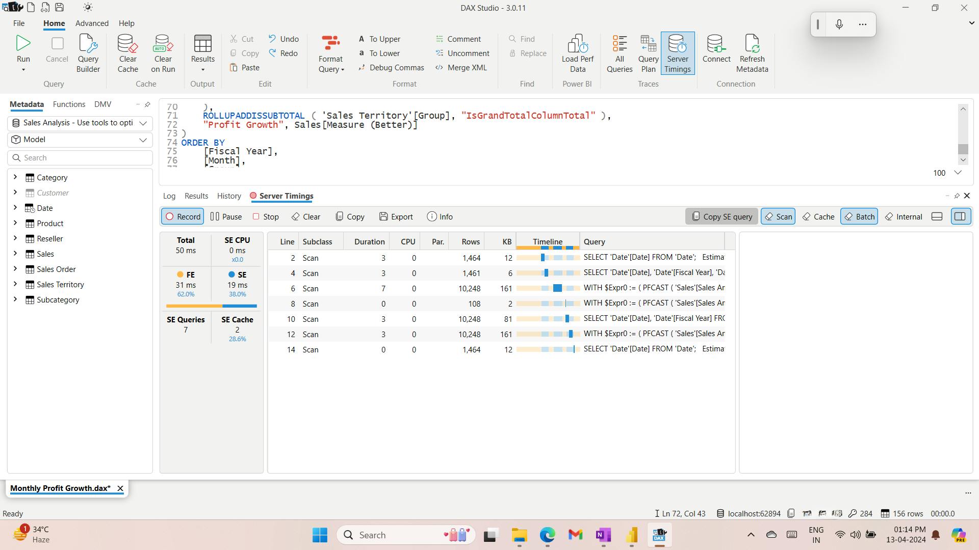
Run it a second time to result in full cache hits.
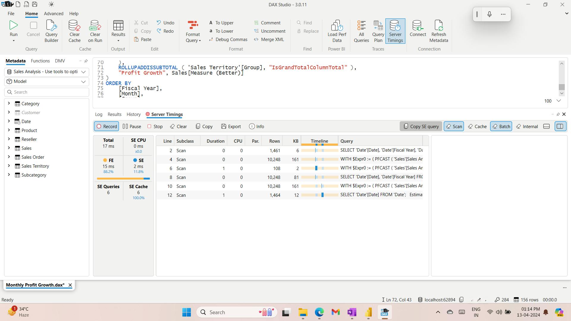
In this case, you can determine that the “better” query, which uses variables and a time intelligence function, performs better-almost a 50% reduction in query execution time.
6. Knowledge check
Stephanie is an enterprise data analyst, working as a resource to data analysts sitting in the finance department. One of the finance analysts asked Stephanie to help troubleshoot why report visuals take 5 seconds to render after a slicer selection is made. What tool should Stephanie use first to begin troubleshooting?
Performance analyzer.
The Performance analyzer is a great tool to start investigating performance issues with visuals in a report.
James has been asked to troubleshoot a report that contains a matrix visual that renders visibly slower than any other visuals on the page. After James runs the Performance analyzer, he notices the need to dig further into the DAX query for the matrix using DAX Studio to understand what's causing the trouble. That same query is running in less than a second in DAX Studio. Has James solved the problem?
No. James needs to clear the model cache to ensure that query results aren't cached in the model.
James may be seeing inaccurate results in either DAX Studio or the Performance analyzer because the query results have been cached.
Mary-Jo is responsible for managing the maintenance and deployment of Power BI assets for the entire organization. What tool can Mary-Jo use to ensure all data models adhere to data modeling best practices?
Best Practice Analyzer in Tabular Editor.
The Best Practice Analyzer in Tabular Editor can be run manually or automated to ensure all models adhere to best practices.
7. Summary
You've been introduced to three tools that you can use to troubleshoot and improve data models.
To optimize a slow report, first you can run the Performance analyzer to measure how each of the report elements performs when users interact with them.
From there, you can dig into DAX query performance in DAX Studio, where you can view, sort, and filter performance data.
You can also troubleshoot single measures or queries and/or evaluate the overall performance of your data model.
To design data models proactively, you can use the Best Practice Analyzer rules in Tabular Editor to implement data modeling best practices as you go.
Performance analyzer helps you understand how report elements like visuals and DAX queries are performing, helps you optimize at two of the four architecture levels, the data model and report visuals.
The Report Canvas retrieves data using a high-level, internal, Power BI query language known as Semantic Query.
DAX queries against tables in Direct Query mode will trigger queries to the Direct Query data source.
As users interact with visuals in Power BI reports, DAX queries are submitted to the dataset and cached into memory. Because of this, you may need to clear the DAX query cache to get accurate results in the Performance analyzer. You can clear the cache by either closing and re-opening your report, or using DAX Studio.
use DAX Studio to investigate your queries in more detail by copying your query from the performance analyzer.
VertiPaq engine - compression algorithms and a multi-threaded query processor
using Tabular Editor to run the BPA to ensure you're implementing data modeling best practices as you build.
When BPA rules are run on your tabular model, you'll get a list of rules that your model violates, and can fix them using Tabular Editor.
install and use Tabular Editor, and DAX Studio to optimize a semantic model.
Learning objectives
After completing this module, you'll be able to:
Optimize queries using performance analyzer.
Troubleshoot DAX performance using DAX Studio.
Optimize a data model using Tabular Editor, using BPA rules.
XII. Create and manage a Power BI deployment pipeline
Deployment pipelines enable creators to develop and test Power BI content in the Power BI service before the content is made available for consumption by users.
It offers creators improved productivity, faster delivery of content updates, and reduced manual work and errors.
The tool is designed as a pipeline with three stages: development, test, and production.
1. Introduction
With increasing consumption, users also demand more from their analytics – more information in a single report, new and easier ways to answer questions, as well as fresh, reliable, and constantly updated data.
2. Understand the deployment process
The Deployment Pipeline tool enables users to manage the development lifecycle of content within their tenant.
Pipelines enable a continuous integration/continuous deployment (CI/CD) approach that ensures content is updated, well-tested, and regularly refreshed as needed.
Pipelines are an efficient and durable way to automate the movement of content (reports, paginated reports, dashboards, semantic models, and dataflows) through the development, test, and production stages of the content development lifecycle:
3. Create a deployment pipeline
i. Create a pipeline from the Deployment pipelines tab
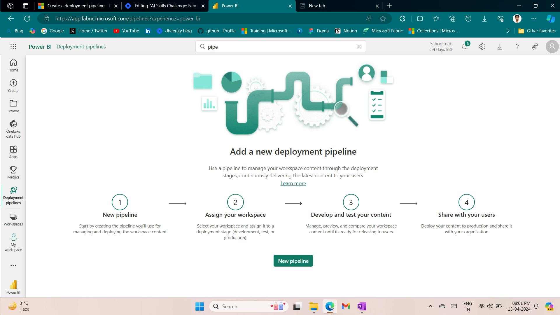
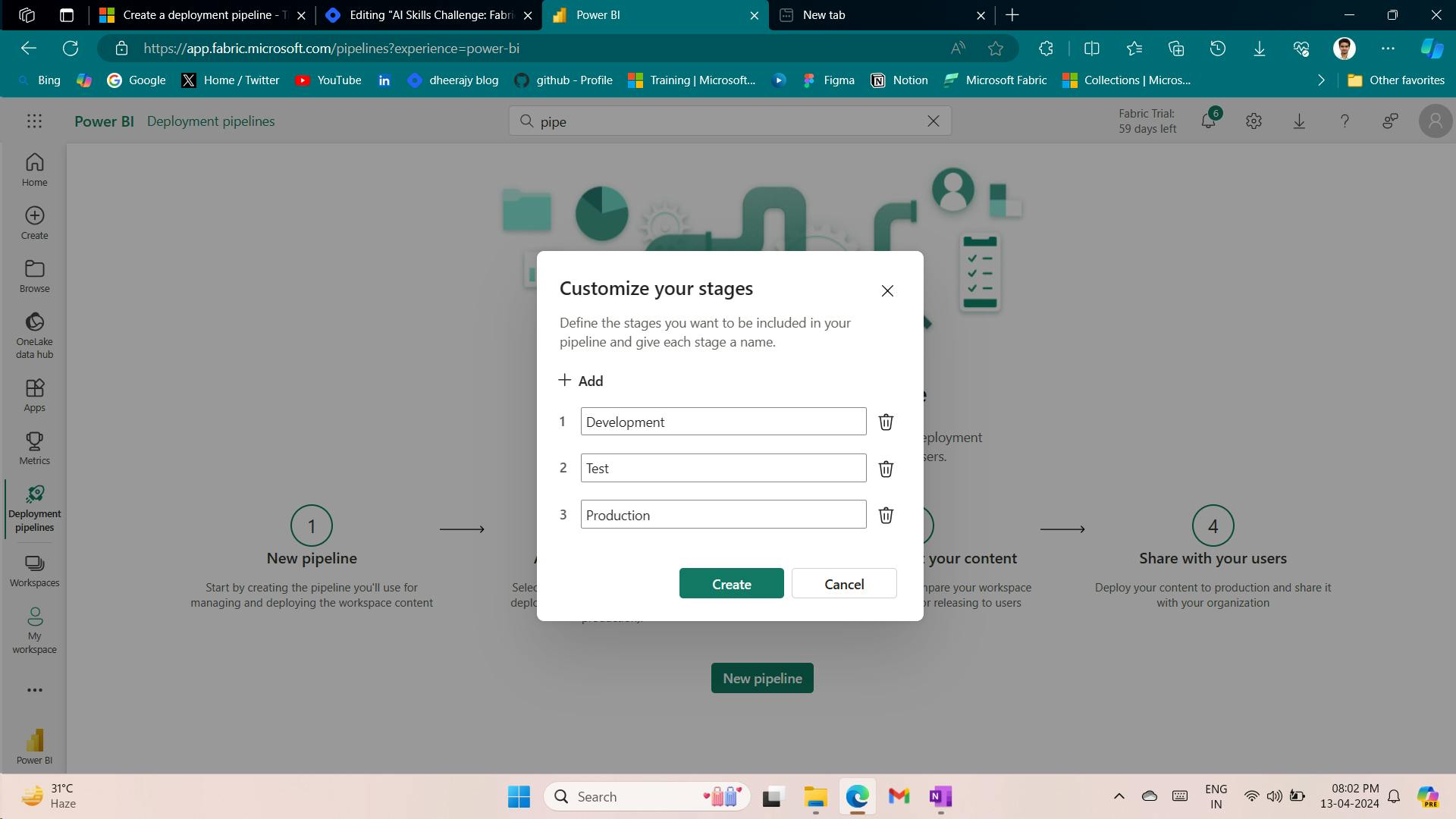
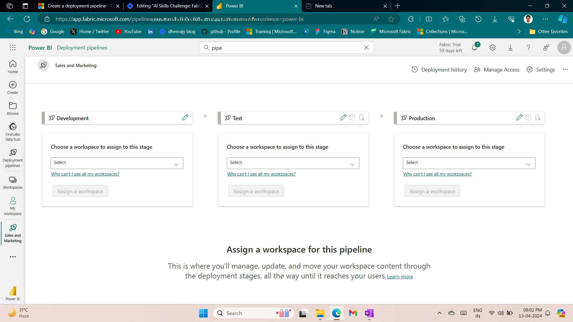
ii. Create a pipeline from a workspace
unable to find.
4. Assign a workspace
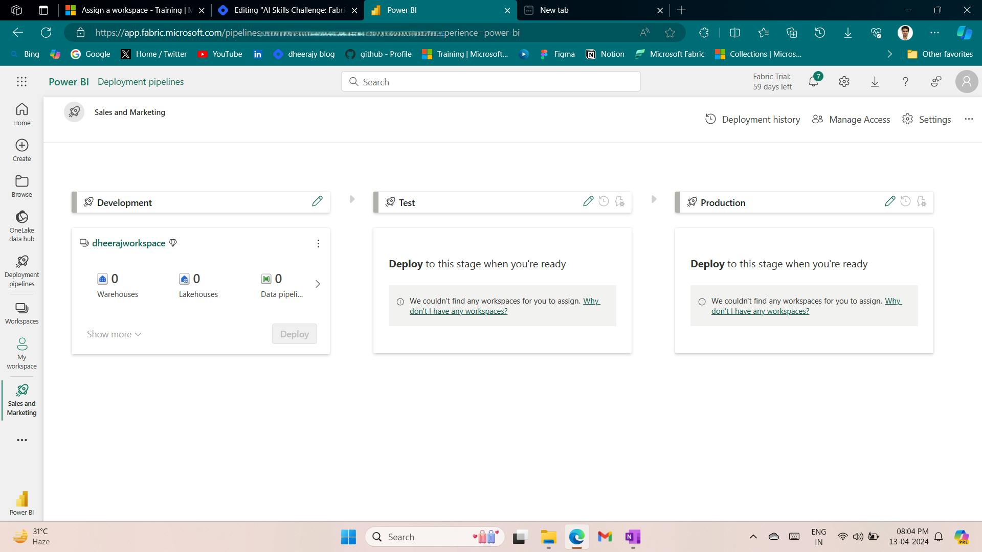
5. Deploy content
The deployment process lets you clone content from one stage in the pipeline to another, typically from development to test, and from test to production.
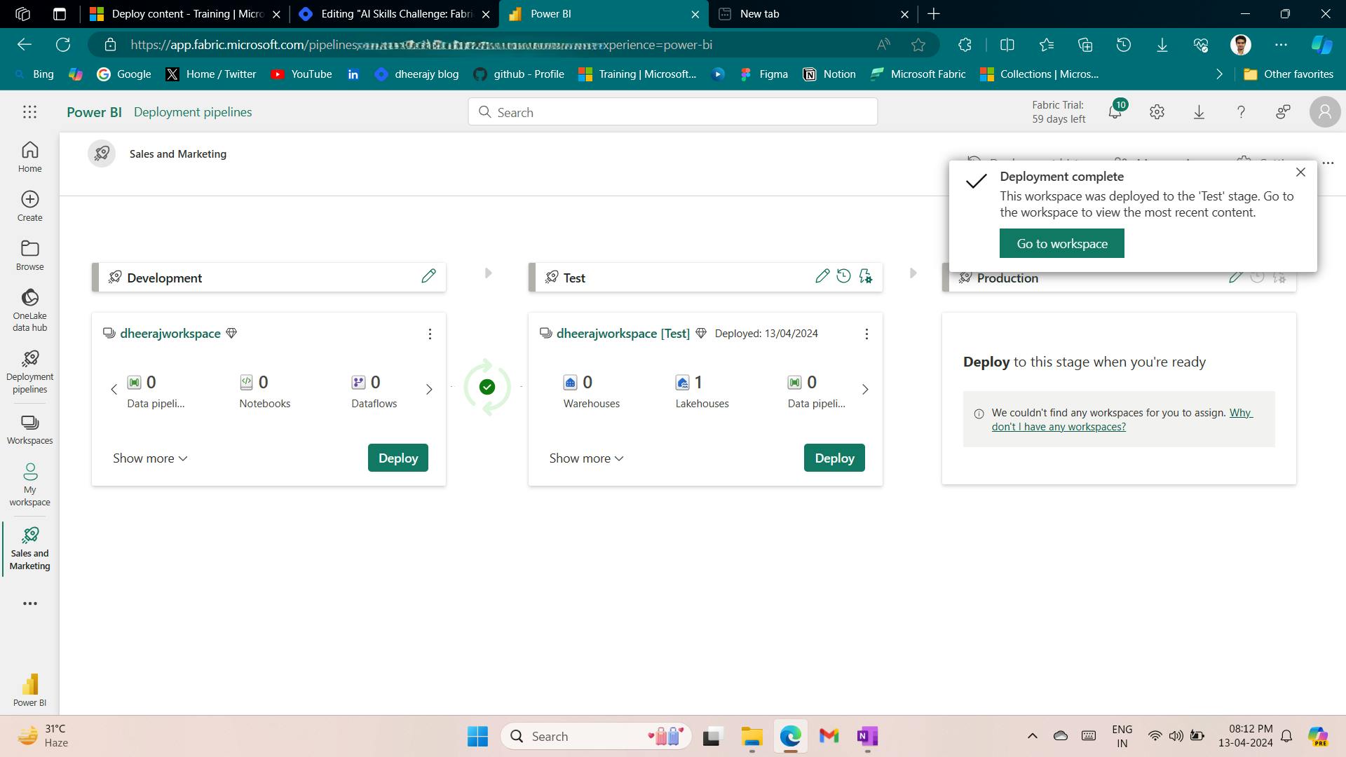
6. Work with deployment pipelines
i. Compare stages
added table
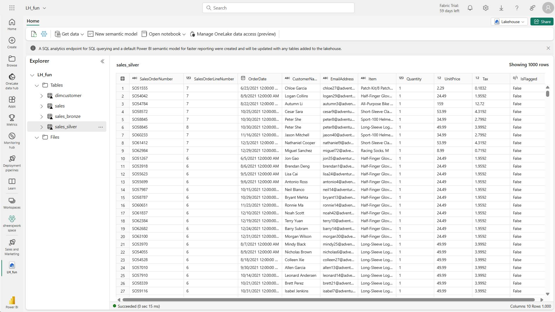
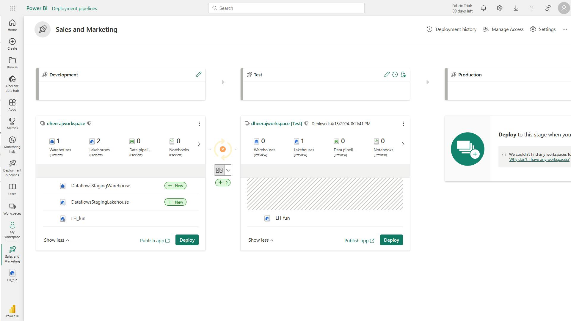
Error:
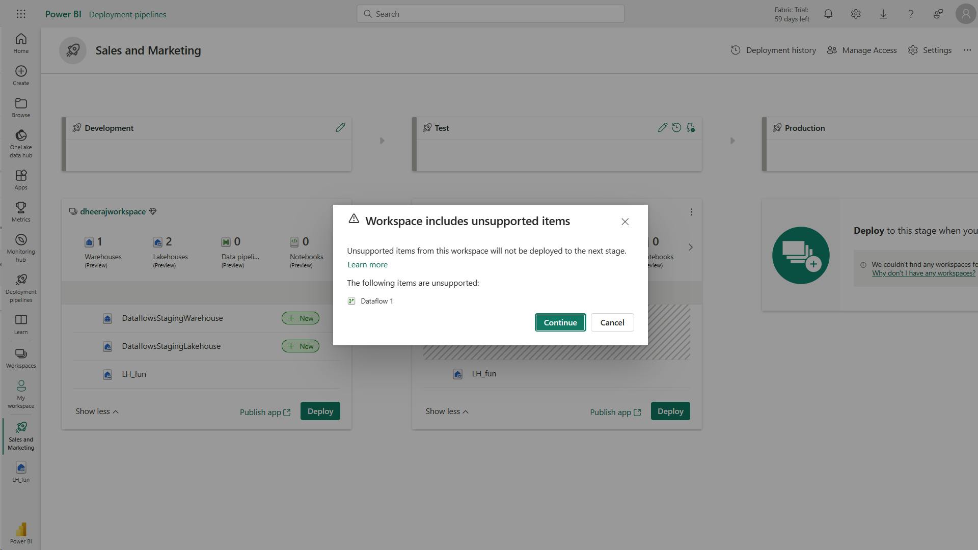
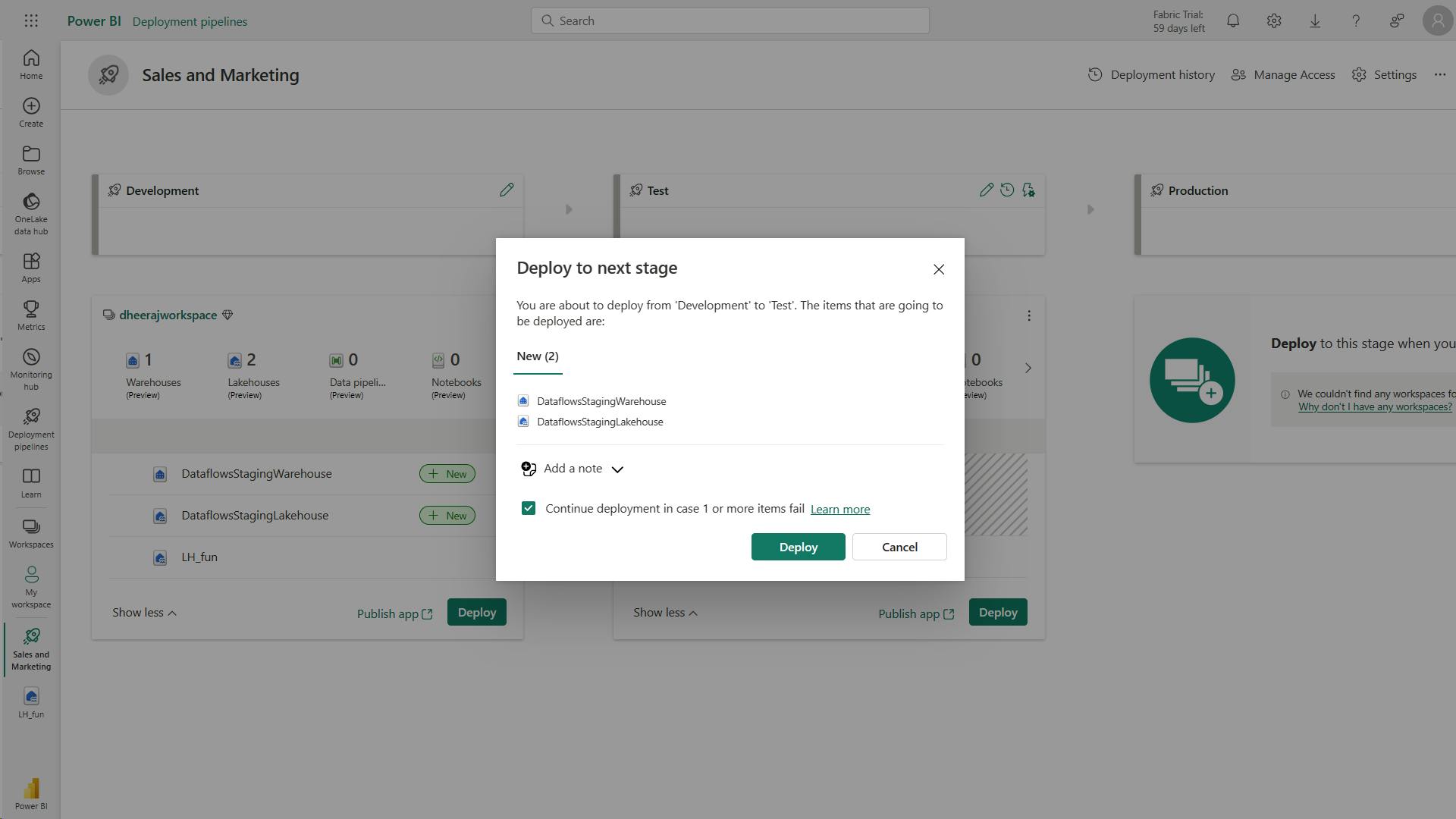
complete:
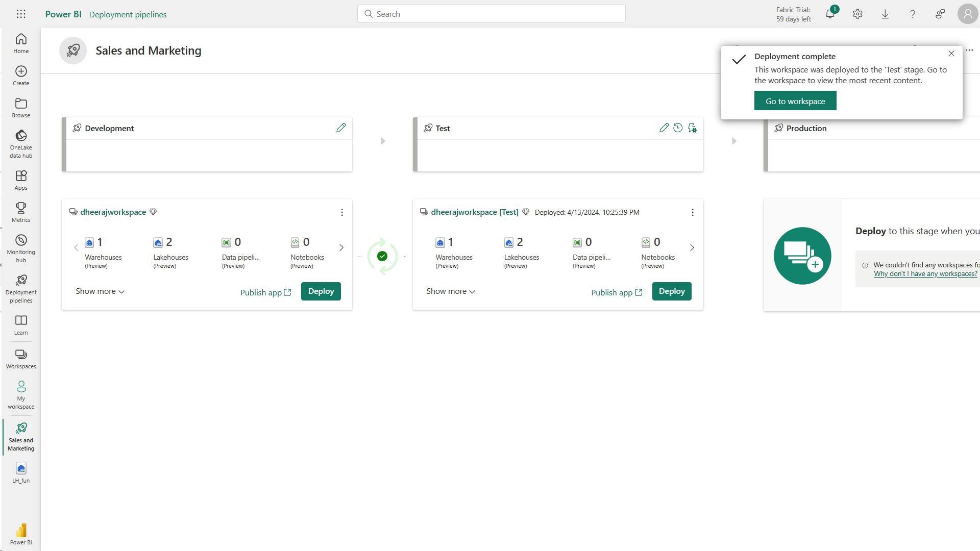
:
ii. Deployment rules enable customization of stages
Configuring deployment rules enables you to allow changes to content when you deploy content between pipeline stages.
For example, if you want a semantic model in a production stage to point to a production database, you can define a rule for semantic model.
The rule is defined in the production stage, under the appropriate semantic model.
Once the rule is defined, content deployed from test to production will inherit the value as defined in the deployment rule, and will always apply it as long as the rule is unchanged and valid.
7. Check your knowledge
Which of the following is a key benefit of deployment pipelines?
Deployment pipelines result in less manual work and fewer errors. They were not designed to help configure semantic models, publish from multiple workspaces, or enhance user access to BI report source data
Correct. Using deployment pipelines leads to less manual work and fewer errors.
After creating a pipeline, what step must you take to add content to your pipeline?
Assign a workspace containing the content you wish to manage in your pipeline.
What is the primary advantage of the Compare view capability between pipeline stages?
Using the Compare view option helps you identify and track changes between items in each pipeline stage.
8. Summary
Power BI deployment pipelines allow you to:
Create multiple Power BI deployment pipelines and share them with others.
Easily deploy content and copy it across Development, Test and Production environments.
Approve/deny the changes or updates made by others for the next deployment pipeline.
Configure the parameter and data source rules settings for each of the environments to keep the connections to the data.
Learning objectives
By the end of this module, you’ll be able to:
Articulate the benefits of deployment pipelines
Create a deployment pipeline using Premium workspaces
Assign and deploy content to pipeline stages, compare
Describe the purpose of deployment rules
Deploy content from one pipeline stage to another
XIII. Administer Microsoft Fabric
Microsoft Fabric is a SaaS solution for end-to-end data analytics. As an administrator, you can configure features and manage access to suit your organization's needs.
1. Introduction
Fabric administrator (admin) - architecture, security and governance features, analytics capabilities, and various deployment and licensing options available
By the end of this module, you'll have an understanding of the Fabric administrator role and the tasks and tools involved in administering Fabric.
2. Understand the Fabric Architecture
Microsoft Fabric - SaaS foundation, simple and integrated approach, all-in-one analytics solution for data movement to data science, real-time analytics, and business intelligence.
Microsoft Fabric - data warehousing, data engineering, data integration, data science, real-time analytics, business intelligence.
Fabric architecture, with OneLake as the foundation, and each experience built on top.
i. Understand Fabric concepts: tenant, capacity, domain, workspace, and item
a. Fabric tenant
create, store, and manage Fabric items.
single instance of Fabric aligned with Microsoft Entra ID.
The Fabric tenant maps to the root of OneLake and is at the top level of the hierarchy.
b. Fabric capacity
Fabric offers capacity through the Fabric SKU and Trials.
c. Fabric domain
is a logical grouping of workspaces.
For example, you might have a domain for sales, another for marketing, and another for finance.
d. Fabric workspace
is a collection of items that brings together different functionality in a single tenant.
For example, in a sales workspace, users associated with the sales organization can create a data warehouse, run notebooks, create semantic models, create reports, etc.
e. Fabric items
different types of items, such as data warehouses, data pipelines, semantic models, reports, and dashboards.
3. Understand the Fabric administrator role
Power BI admin role - Fabric admin.
i. Describe admin tasks
Security and access control: RBAC, data gateways
Data governance: inbound and outbound connectivity
Customization and configuration: configuring private links, defining data classification policies
Monitoring and optimization: configuring monitoring and alerting settings, optimizing query performance, managing capacity and scaling, and troubleshooting data refresh and connectivity issues
ii. Describe admin tools
Fabric admins can perform most admin tasks using the tools: the Fabric admin portal, PowerShell cmdlets, admin APIs and SDKs, and the admin monitoring workspace.
a. Fabric admin portal
b. PowerShell cmdlets
c. Admin APIs and SDKs
An admin API and SDK are tools that allow developers to interact with a software system programmatically.
An API (Application Programming Interface) is a set of protocols and tools that enable communication between different software applications.
An SDK (Software Development Kit) is a set of tools and libraries that helps developers create software applications that can interact with a specific system or platform.
You can use APIs and SDKs to automate common administrative tasks and integrate Fabric with other systems.
d. Admin monitoring workspace
4. Manage Fabric security
Microsoft Fabric security is based on Power BI security.
i. Manage users: assign and manage licenses
License management for Fabric is handled in the Microsoft 365 admin center.
ii. Manage items and sharing
Items in workspaces are best distributed through a workspace app or the workspace directly.
Granting the least permissive rights is the first step is securing the data.
5. Govern data in Fabric
Endorsement is a way for you as an admin to designate specific Fabric items as trusted and approved for use across the organization.
Admins can also make use of the scanner API to scan Fabric items for sensitive data, and the data lineage feature to track the flow of data through Fabric.
i. Endorse Fabric content
Content endorsement is an essential governance feature that helps you establish trust in your data assets by promoting and certifying specific Fabric items as trusted and approved for use across the organization. All Fabric items can be endorsed except dashboards.
Endorsed assets are identified with a badge that indicates they have been reviewed and approved. Endorsement helps your users know which assets they can trust and rely on for accurate information
Promoted Fabric content appears with a Promoted badge in the Fabric portal. Workspace members with the contributor or admin role can promote content within a workspace. The Fabric admin can promote content across the organization.
ii. Scan for sensitive data
Metadata scanning facilitates governance of data by enabling cataloging and reporting on all the metadata of your organization's Fabric items.
The scanner API is a set of Admin REST APIs that allows you to scan Fabric items for sensitive data. Use the scanner API to scan data warehouses, data pipelines, semantic models, reports, and dashboards for sensitive data. The scanner API can be used to scan both structured and unstructured data.
iii. Track data lineage
Data lineage is the ability to track the flow of data through Fabric. Data lineage allows you to see where data comes from, how it's transformed, and where it goes. This helps you understand the data that is available in Fabric, and how it's being used.
6. Knowledge check
Which of the following statements best describes the concept of capacity in Fabric?
Capacity defines the ability of a resource to perform an activity or to produce output.
Capacity refers to the resources available at a given time to perform activities and produce output.
Which of the following statements is true about the difference between promotion and certification in Fabric?
Certification must be enabled in the tenant by the admin, while promotion can be done by a workspace member.
Certification must be enabled in the tenant by the admin, and only designated certifiers can perform the endorsement. In contrast, promotion can be done by any workspace member who has been granted the necessary permissions.
7. Summary
In this module,
you learned about the Fabric architecture and the role of an admin in managing the Fabric platform.
You also explored the different tools available for managing security and sharing, as well as the governance features that can be used to enforce standards and ensure compliance.
Your understanding of how to manage a Fabric environment ensures that it is secure, compliant, and well-governed.
With this knowledge, you are well-equipped to help your organization get the most out of Fabric and derive valuable insights from all your data.
Fabric administrator (admin) - architecture, security and governance features, analytics capabilities, and various deployment and licensing options available
tenant, capacity, domain, workspace, and item
Fabric admin tasks - Security and access control(RBAC, data gateways), Data governance(inbound and outbound connectivity), Customization and configuration, Monitoring and optimization,
Fabric admins can perform most admin tasks using the tools: the Fabric admin portal, PowerShell cmdlets, admin APIs and SDKs, and the admin monitoring workspace.
License management for Fabric is handled in the Microsoft 365 admin center
Endorsed assets - reviewed and approved, can trust and rely on for accurate information
Promoted Fabric content - contributor or admin role can promote content within a workspace. The Fabric admin can promote content across the organization.
The scanner API - Admin REST APIs, scan Fabric items for sensitive data, scan data warehouses, data pipelines, semantic models, reports, and dashboards for sensitive data, scan both structured and unstructured data.
Data lineage - to track the flow of data, see where data comes from, how it's transformed, and where it goes.
Learning objectives
In this module, you'll learn how to:
Describe Fabric admin tasks
Navigate the admin center
Manage user access
I Completed AI Skills Challenge: Fabric Analytics Engineer journey! in 9 days.
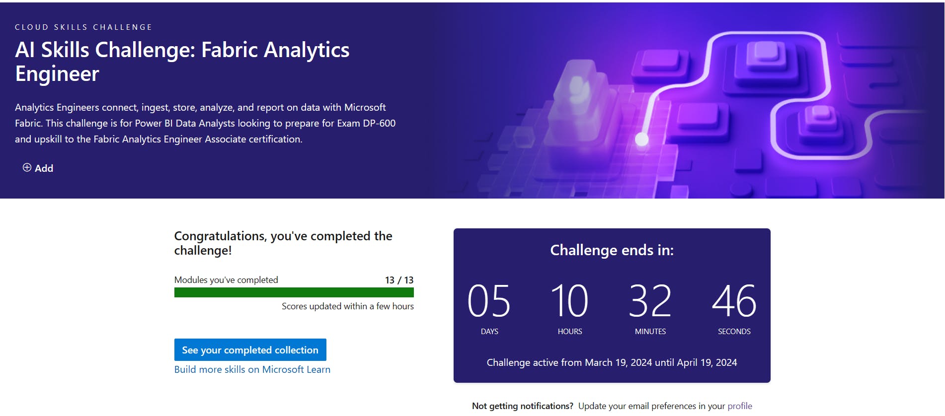
Conclusion
Learning Objectives,
Describe end-to-end analytics in Microsoft Fabric
Get started with lakehouses in Microsoft Fabric
Use Apache Spark in Microsoft Fabric
Work with Delta Lake tables in Microsoft Fabric
Use Data Factory pipelines in Microsoft Fabric
Ingest Data with Dataflows Gen2 in Microsoft Fabric
Ingest data with Spark and Microsoft Fabric notebooks
Organize a Fabric lakehouse using medallion architecture design
Get started with data warehouses in Microsoft Fabric
Load data into a Microsoft Fabric data warehouse
Use tools to optimize Power BI performance
Create and manage a Power BI deployment pipeline
Administer Microsoft Fabric
and Exercises completed:
Create and ingest data with a Microsoft Fabric lakehouse
Analyze data with Apache Spark
Use delta tables in Apache Spark
Ingest data with a pipeline
Create and use a Dataflow Gen2 in Microsoft Fabric
Ingest data with Spark and Microsoft Fabric notebooks
Organize your Fabric lakehouse using a medallion architecture notebook to transform the data, Upsert operation on a Delta table
Analyze data in a data warehouse
Load data into a warehouse in Microsoft Fabric
use two external tools to help you develop, manage, and optimize data models and DAX queries.
Create a deployment pipeline